
In this tutorial, we will write a program to correct camera lens distortion using OpenCV. This process is known as camera calibration.
Real-World Applications
- Self-Driving Cars
- Robotics (Translating Between Real-World Coordinates and Camera Coordinates)
Prerequisites
Install OpenCV
The first thing you need to do is to make sure you have OpenCV installed on your machine. If you are using Anaconda, you can type:
conda install -c conda-forge opencv
Alternatively, you can type:
pip install opencv-python
What Is Camera Calibration and Why Is It Important?
A camera’s job is to convert light that hits its image sensor into an image. An image is made up of picture elements known as pixels.
In a perfect world, these pixels (i.e. what the camera sees) would look exactly like what you see in the real world. However, no camera is perfect. They all contain physical flaws that can, in some cases, cause significant distortion.
For example, look at an extreme example of image distortion below.
Here is the same image after calibrating the camera and correcting for the distortion.
Do you see how this could lead to problems…especially in robotics where accuracy key?
Imagine you have a robotic arm that is working inside a warehouse. Its job is to pick up items off a conveyor belt and place those items into a bin.
To help the robot determine the exact position of the items, there is a camera overhead. To get an accurate translation between camera pixel coordinates and real world coordinates, you need to calibrate the camera to remove any distortion.
The two most important forms of distortion are radial distortion and tangential distortion.
Radial distortion occurs when straight lines appear curved. Here is an example below of a type of radial distortion known as barrel distortion. Notice the bulging in the image that is making straight lines (in the real world) appear curved.

Tangential distortion occurs when the camera lens is not exactly aligned parallel to the camera sensor. Tangential distortion can make the real world look stretched or tilted. It can also make items appear closer than they are in real life.
To get an accurate representation of the real world on a camera, we have to calibrate the camera. We want to know that when we see an object of a certain size in the real world, this size translates to a known size in camera pixel coordinates.
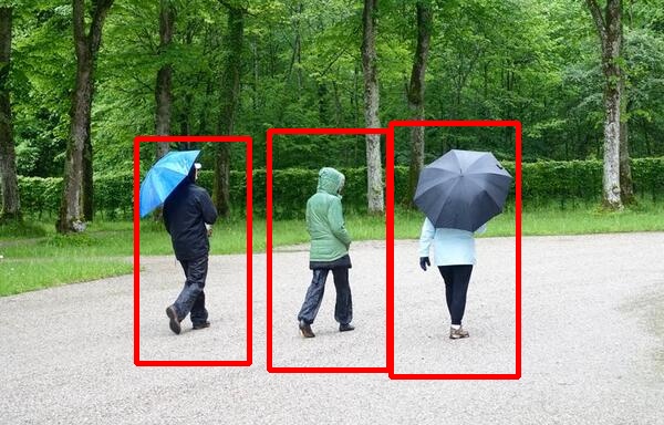
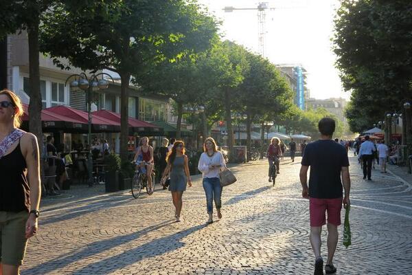
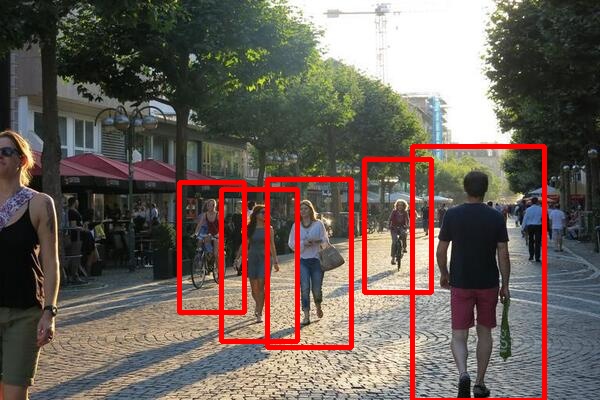
By calibrating a camera, we can enable a robotic arm, for example, to have better “hand-eye” coordination. You also enable a self-driving car to know the location of pedestrians, dogs, and other objects relative to the car.
Calibrating the camera is the process of using a known real-world pattern (e.g. a chessboard) to estimate the extrinsic parameters (rotation and translation vectors) and intrinsic parameters (e.g. focal length, optical center, etc.) of a camera’s lens and image sensor to reduce distortion error caused by the camera’s imperfections.
These parameters include:
- Focal length
- Image (i.e. optical) center (it is usually not exactly at (width/2, height/2))
- Scaling factors for the pixels along the rows and columns
- Skew factor
- Lens distortion
Why Use a Chessboard?
Chessboard calibration is a standard technique for performing camera calibration and estimating the values of the unknown parameters I mentioned in the previous section.
OpenCV has a chessboard calibration library that attempts to map points in 3D on a real-world chessboard to 2D camera coordinates. This information is then used to correct distortion.
Note that any object could have been used (a book, a laptop computer, a car, etc.), but a chessboard has unique characteristics that make it well-suited for the job of correcting camera distortions:
- It is flat, so you don’t need to deal with the z-axis (z=0), only the x and y-axis. All the points on the chessboard lie on the same plane.
- There are clear corners and points, making it easy to map points in the 3D real world coordinate system to points on the camera’s 2D pixel coordinate system.
- The points and corners all occur on straight lines.
Perform Camera Calibration Using OpenCV
The official tutorial from OpenCV is here on their website, but let’s go through the process of camera calibration slowly, step by step.
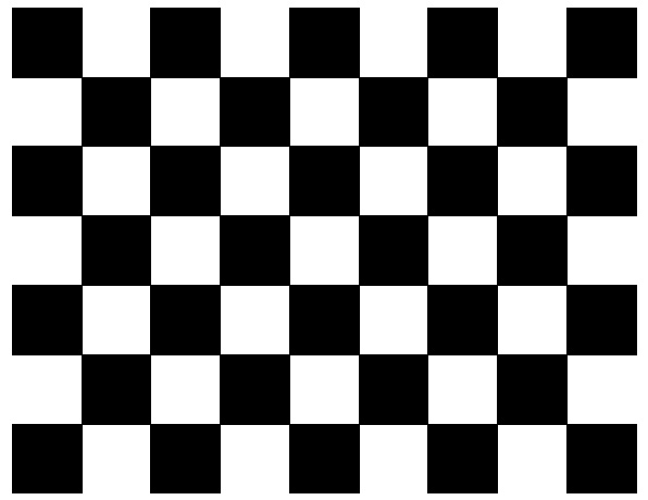
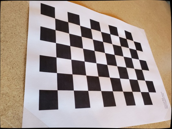
Print a Chessboard
The first step is to get a chessboard and print it out on regular A4 size paper. You can download this pdf, which is the official chessboard from the OpenCV documentation, and just print that out.
Measure Square Length
Measure the length of the side of one of the squares. In my case, I measured 2.3 cm (0.023 m).
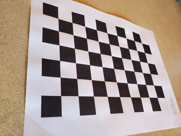
Take Photos of the Chessboard From Different Distances and Orientations
We need to take at least 10 photos of the chessboard from different distances and orientations. I’ll take 19 photos so that my algorithm will have a lot of input images from which to perform camera calibration.
Tape the chessboard to a flat, solid object.
Take the photos, and then move them to a directory on your computer.
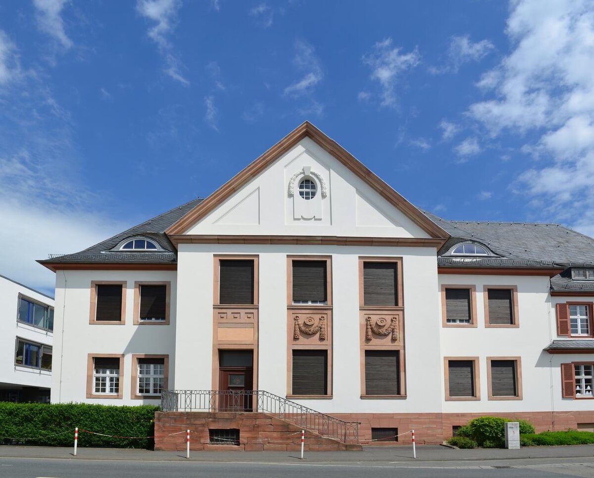
Here are examples of some of the photos I took:
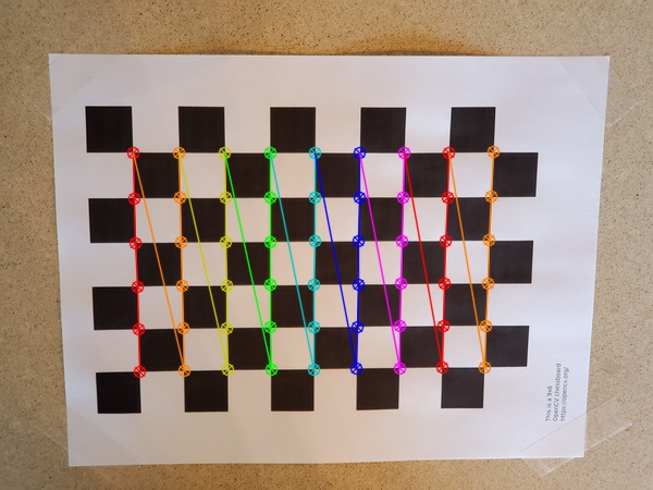
Draw the Corners
The first thing we need to do is to find and then draw the corners on the image.
Make sure you have NumPy installed, a scientific computing library for Python.
If you’re using Anaconda, you can type:
conda install numpy
Alternatively, you can type:
pip install numpy
Write the following code in Python. You can copy and paste this code into your favorite IDE. Pick one of the chessboard images as a test case. I’ll name the file draw_corners.py. This code will draw the corners on an input chessboard image and then save the drawing to an image file.
import cv2 # Import the OpenCV library to enable computer vision
import numpy as np # Import the NumPy scientific computing library

# Author: Addison Sears-Collins
# https://automaticaddison.com
# Description: Detect corners on a chessboard

filename = 'chessboard_input1.jpg'

# Chessboard dimensions
number_of_squares_X = 10 # Number of chessboard squares along the x-axis
number_of_squares_Y = 7  # Number of chessboard squares along the y-axis
nX = number_of_squares_X - 1 # Number of interior corners along x-axis
nY = number_of_squares_Y - 1 # Number of interior corners along y-axis

def main():

  # Load an image
  image = cv2.imread(filename)

  # Convert the image to grayscale
  gray = cv2.cvtColor(image, cv2.COLOR_BGR2GRAY)

  # Find the corners on the chessboard
  success, corners = cv2.findChessboardCorners(gray, (nY, nX), None)

  # If the corners are found by the algorithm, draw them
  if success == True:

    # Draw the corners
    cv2.drawChessboardCorners(image, (nY, nX), corners, success)

    # Create the output file name by removing the '.jpg' part
    size = len(filename)
    new_filename = filename[:size - 4]
    new_filename = new_filename + '_drawn_corners.jpg'

    # Save the new image in the working directory
    cv2.imwrite(new_filename, image)

    # Display the image
    cv2.imshow("Image", image)

    # Display the window until any key is pressed
    cv2.waitKey(0)

    # Close all windows
    cv2.destroyAllWindows()

main()
Run the code.
Here is the output:

Write the Python Code for Camera Calibration
Now that we know how to identify corners on a chessboard, let’s write the code to perform camera calibration.
Here is the code. I put my distorted image inside a folder named ‘distorted’ inside the working directory. This folder is where the output undistorted saves to.
Don’t be scared at how long the code is. I put a lot of comments in here in order to make each line easier for you to understand. Just copy and paste the code into your favorite text editor or IDE. I named the file camera_calibration.py.
# Author: Addison Sears-Collins
# https://automaticaddison.com
# Description: Perform camera calibration using a chessboard.

import cv2 # Import the OpenCV library to enable computer vision
import numpy as np # Import the NumPy scientific computing library
import glob # Used to get retrieve files that have a specified pattern

# Path to the image that you want to undistort
distorted_img_filename = 'distorted/chessboard_input12.jpg'

# Chessboard dimensions
number_of_squares_X = 10 # Number of chessboard squares along the x-axis
number_of_squares_Y = 7  # Number of chessboard squares along the y-axis
nX = number_of_squares_X - 1 # Number of interior corners along x-axis
nY = number_of_squares_Y - 1 # Number of interior corners along y-axis
square_size = 0.023 # Length of the side of a square in meters

# Store vectors of 3D points for all chessboard images (world coordinate frame)
object_points = []

# Store vectors of 2D points for all chessboard images (camera coordinate frame)
image_points = []

# Set termination criteria. We stop either when an accuracy is reached or when
# we have finished a certain number of iterations.
criteria = (cv2.TERM_CRITERIA_EPS + cv2.TERM_CRITERIA_MAX_ITER, 30, 0.001)

# Define real world coordinates for points in the 3D coordinate frame
# Object points are (0,0,0), (1,0,0), (2,0,0) ...., (5,8,0)
object_points_3D = np.zeros((nX * nY, 3), np.float32)

# These are the x and y coordinates
object_points_3D[:,:2] = np.mgrid[0:nY, 0:nX].T.reshape(-1, 2)

object_points_3D = object_points_3D * square_size

def main():

  # Get the file path for images in the current directory
  images = glob.glob('*.jpg')

  # Go through each chessboard image, one by one
  for image_file in images:

    # Load the image
    image = cv2.imread(image_file)

    # Convert the image to grayscale
    gray = cv2.cvtColor(image, cv2.COLOR_BGR2GRAY)

    # Find the corners on the chessboard
    success, corners = cv2.findChessboardCorners(gray, (nY, nX), None)

    # If the corners are found by the algorithm, draw them
    if success == True:

      # Append object points
      object_points.append(object_points_3D)

      # Find more exact corner pixels
      corners_2 = cv2.cornerSubPix(gray, corners, (11,11), (-1,-1), criteria)

	  # Append image points
      image_points.append(corners_2)

      # Draw the corners
      cv2.drawChessboardCorners(image, (nY, nX), corners_2, success)

      # Display the image. Used for testing.
      #cv2.imshow("Image", image)

      # Display the window for a short period. Used for testing.
      #cv2.waitKey(200)

  # Now take a distorted image and undistort it
  distorted_image = cv2.imread(distorted_img_filename)

  # Perform camera calibration to return the camera matrix, distortion coefficients, rotation and translation vectors etc
  ret, mtx, dist, rvecs, tvecs = cv2.calibrateCamera(object_points,
                                                    image_points,
                                                    gray.shape[::-1],
                                                    None,
                                                    None)

  # Get the dimensions of the image
  height, width = distorted_image.shape[:2]

  # Refine camera matrix
  # Returns optimal camera matrix and a rectangular region of interest
  optimal_camera_matrix, roi = cv2.getOptimalNewCameraMatrix(mtx, dist,
                                                            (width,height),
                                                            1,
                                                            (width,height))

  # Undistort the image
  undistorted_image = cv2.undistort(distorted_image, mtx, dist, None,
                                    optimal_camera_matrix)

  # Crop the image. Uncomment these two lines to remove black lines
  # on the edge of the undistorted image.
  #x, y, w, h = roi
  #undistorted_image = undistorted_image[y:y+h, x:x+w]

  # Display key parameter outputs of the camera calibration process
  print("Optimal Camera matrix:")
  print(optimal_camera_matrix)

  print("\n Distortion coefficient:")
  print(dist)

  print("\n Rotation Vectors:")
  print(rvecs)

  print("\n Translation Vectors:")
  print(tvecs)

  # Create the output file name by removing the '.jpg' part
  size = len(distorted_img_filename)
  new_filename = distorted_img_filename[:size - 4]
  new_filename = new_filename + '_undistorted.jpg'

  # Save the undistorted image
  cv2.imwrite(new_filename, undistorted_image)

  # Close all windows
  cv2.destroyAllWindows()

main()
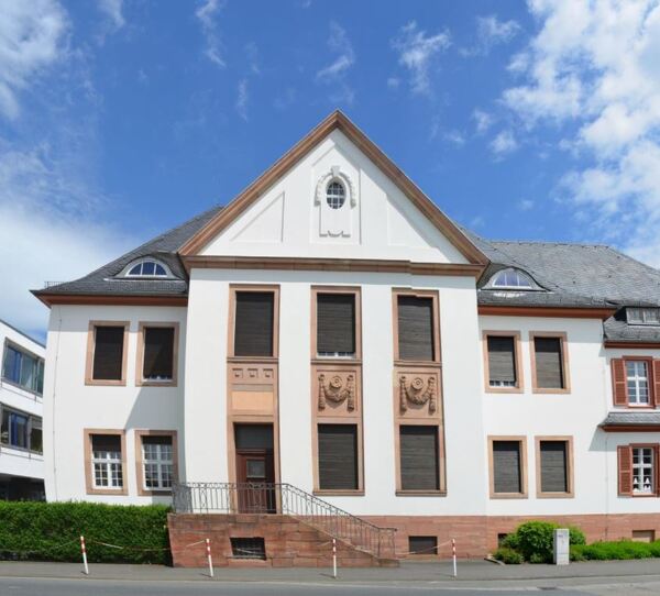
Output
Here is the original distorted image.
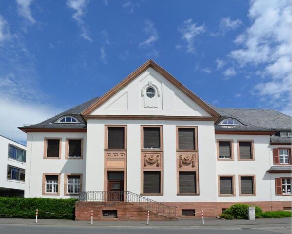
Here is the undistorted image, which is the output. Note that the distorted image is the same dimensions as the undistorted image. Both images are 600 x 450 pixels.
The correction is quite subtle, so it might be hard to see (my camera must be pretty good!). It is more noticeable when I flip back and forth between both images as you see in the gif below.
Saving Parameters Using Pickle
If you want to save the camera calibration parameters to a file, you can use a package like Pickle to do it. It will encode these parameters into a text file that you can later upload into a program.
The three key parameters you want to make sure to save are mtx, dist, and optimal_camera_matrix.
Here is a list of some tutorials on how to use Pickle:
Assuming you have import pickle at the top of your program, the Python code for saving the parameters to a pickle file would be as follows:
# Save the camera calibration results.
calib_result_pickle = {}
calib_result_pickle["mtx"] = mtx
calib_result_pickle["optimal_camera_matrix"] = optimal_camera_matrix
calib_result_pickle["dist"] = dist
calib_result_pickle["rvecs"] = rvecs
calib_result_pickle["tvecs"] = tvecs
pickle.dump(calib_result_pickle, open("camera_calib_pickle.p", "wb" ))
Then if at a later time, you wanted to load the parameters into a new program, you would use this code:
calib_result_pickle = pickle.load(open("camera_calib_pickle.p", "rb" ))
mtx = calib_result_pickle["mtx"]
optimal_camera_matrix = calib_result_pickle["optimal_camera_matrix"]
dist = calib_result_pickle["dist"]
Then, given an input image or video frame (i.e. distorted_image), we can undistort it using the following lines of code:
undistorted_image = cv2.undistort(distorted_image, mtx, dist, None,
                                    optimal_camera_matrix)
That’s it for this tutorial. Hope you enjoyed it. Now you know how to calibrate a camera using OpenCV.
Keep building!
