In this section, we will learn how to work with homogeneous transformation matrices. Homogeneous transformation matrices enable us to combine rotation matrices (which have 3 rows and 3 columns) and displacement vectors (which have 3 rows and 1 column) into a single matrix. They are an important concept of forward kinematics.

Forward kinematics asks the question: Where is the end effector of a robot (e.g. gripper, hand, vacuum suction cup, etc.) located in space given that we know the angles of the servo motors?

Table of Contents

Getting Started

Back when we examined rotation matrices, you remember that we were able to convert the end effector frame into the base frame using matrix multiplication.

rot_mat_0_3 = (rot_mat_0_1)(rot_mat_1_2)(rot_mat_2_3)

However, for displacement vectors, it doesn’t work like this. We can’t just multiply displacement vectors together to calculate the displacement of the end effector frame relative to the base frame.

disp_vec_0_3 ≠ (disp_vec_0_1)(disp_vec_1_2)(disp_vec_2_3)

Homogeneous transformation matrices combine both the rotation matrix and the displacement vector into a single matrix. You can multiply two homogeneous matrices together just like you can with rotation matrices.

For example, let homgen_0_2, mean the homogeneous transformation matrix from frame 0 to frame 2. To calculate it, we can multiply the homogeneous transformation matrix from frame 0 to 1 by the homogeneous transformation matrix from frame 1 to 2:

homgen_0_2 = (homgen_0_1)(homgen_1_2)

A homogeneous transformation takes the following form:

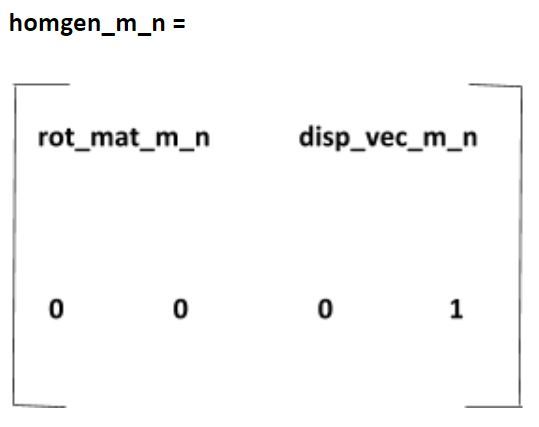
The rotation matrix in the upper left is a 3×3 matrix (i.e. 3 rows by 3 columns), and the displacement vector on the right is 3×1. The matrix above has four rows and four columns in total.

We have to add that bottom row with [0 0 0 1] in order to make the matrix multiplication work out. This addition is standard for homogeneous transformation matrices.

For example, imagine if the homogeneous transformation matrix only had the 3×3 rotation matrix in the upper left and the 3 x 1 displacement vector to the right of that, you would have a 3 x 4 homogeneous transformation matrix (3 rows by 4 column). You can’t multiply two 3×4 matrices together due to the rules of matrix multiplication (the number of columns in the first matrix must be equal to the number of rows in the second matrix).

Adding [0 0 0 1] to the bottom row, makes homogeneous transformation matrices 4×4 (4 rows by 4 columns). And the product formed, by multiplying any two 4×4 matrices that have [0 0 0 1] in the bottom row, is a 4×4 matrix with [0 0 0 1] in the bottom row….so you get standardization across all homogeneous transformation matrices.

Example – Two Degree of Freedom Robotic Arm

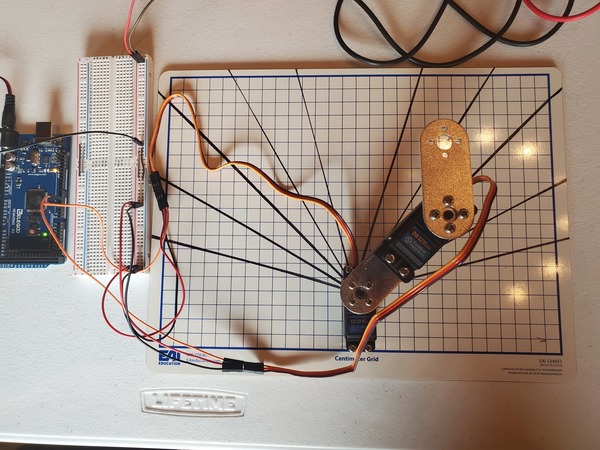
For this example, you need to have already built the 2DOF robotic arm, if you want to follow along with a real robot.

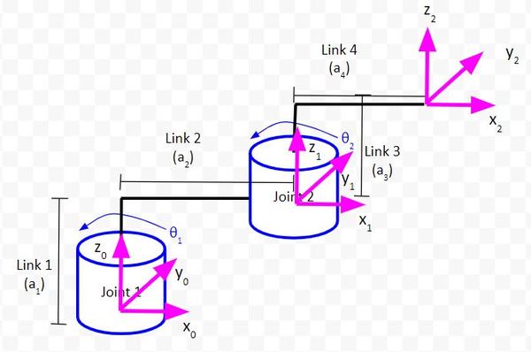
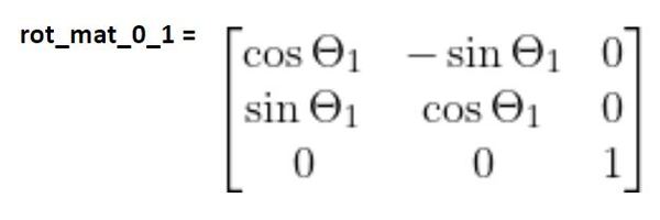
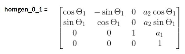
When we made the kinematic diagram for the two degree of freedom manipulator above, we found the following rotation matrices and displacement vector between frame 0 and frame 1:

2-rotation-matrices-displacement-vectorJPG

These matrices above would yield the following homogeneous transformation matrix:

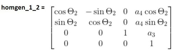
Here is what we had for frame 1 to frame 2:

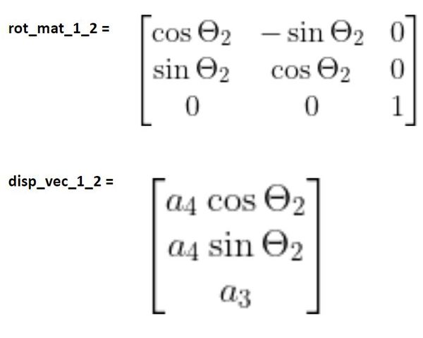
These two matrices would yield the following homogeneous transformation matrix:

The cool thing is we can multiply the two homogeneous transformation matrices above to find the homogeneous transformation matrix from frame 0 to frame 2.

homgen_0_2 = (homgen_0_1)(homgen_1_2)

Once we have our homogeneous transformation matrix, we can pull out the displacement vector to find the position of the end effector relative to the base frame.

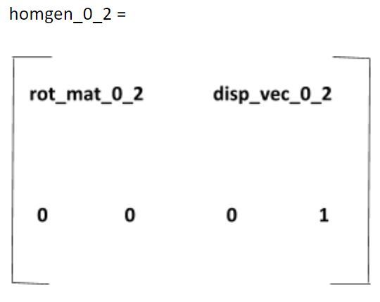
Homogeneous Transformation Matrix From Frame 0 to Frame 2

Let’s see if we can determine the position of the end-effector by calculating the homogeneous transformation matrix from frame 0 to frame 2 of our two degree of freedom robotic manipulator.

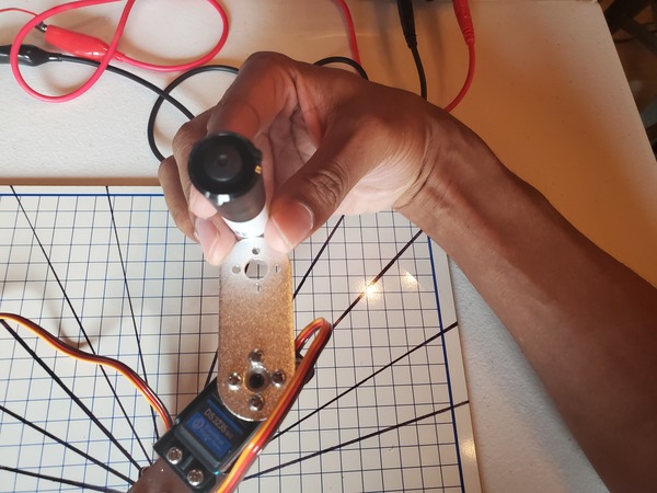
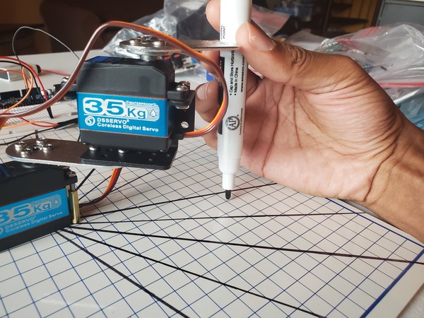
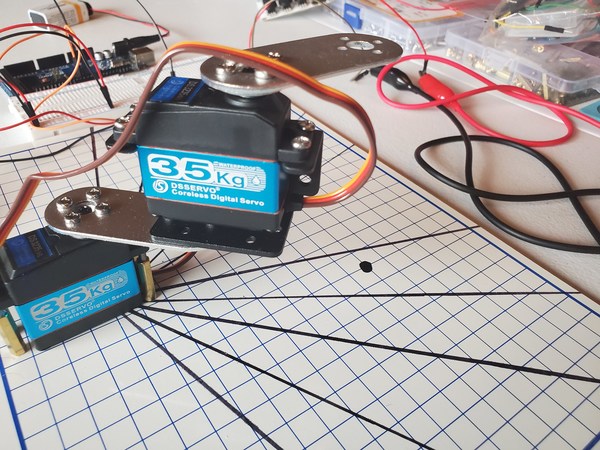
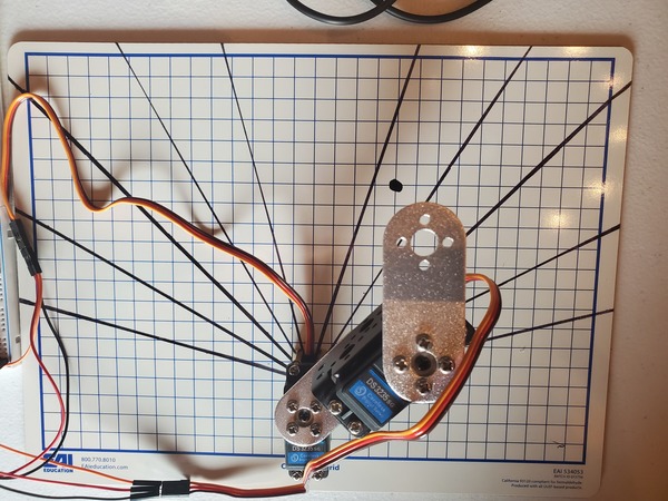
Measure the Link Lengths

Using a ruler, measure the four link lengths.

To measure a₄, hold a dry erase marker vertically so that the tip of the marker touches the dry erase board, and the shaft of the market touches the end of the end effector (i.e. the top beam mount). You will need to measure a₄from the center of the servo horn to the center of the market. Why add the dry erase market? You’ll see why later in this tutorial.

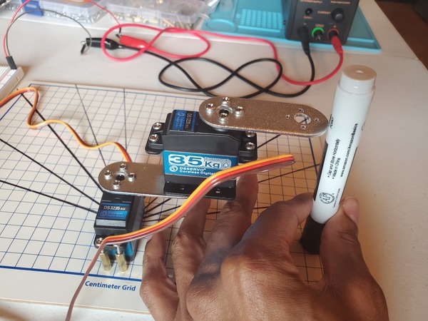
Here are the values I measured for the link lengths:

a₁= 4.7 cm (measured from the top of the dry erase board to the top of the screw of the first servo horn)
a₂ = 5.9 cm (measured from the center of the first servo horn screw across to the center of the second servo horn screw)
a₃ = 5.4 cm (measured from the top of the beam mount to the top of the second servo horn screw)
a₄ = 6.0 cm (measured from the center of the second servo horn screw across to the tip of the dry erase marker that you “attached” to the end of the upper beam mount end effector)

Write the Python Code

Let’s enter all of this into our code. In this example, θ₁ = 45 degrees, and θ₂ = 45 degrees.

Here is the code. I named the file homogeneous_transform_0_2.py:

import numpy as np # Scientific computing library

# Project: Homogeneous Transformation Matrices for a 2 DOF Robotic Arm
# Author: Addison Sears-Collins
# Date created: August 11, 2020

# Servo (joint) angles in degrees
servo_0_angle = 45 # Joint 1
servo_1_angle = 45 # Joint 2

# Link lengths in centimeters
a1 = 4.7 # Length of link 1
a2 = 5.9 # Length of link 2
a3 = 5.4 # Length of link 3
a4 = 6.0 # Length of link 4

# Convert servo angles from degrees to radians
servo_0_angle = np.deg2rad(servo_0_angle)
servo_1_angle = np.deg2rad(servo_1_angle)

# Define the first rotation matrix.
# This matrix helps convert servo_1 frame to the servo_0 frame.
# There is only rotation around the z axis of servo_0.
rot_mat_0_1 = np.array([[np.cos(servo_0_angle), -np.sin(servo_0_angle), 0],
                        [np.sin(servo_0_angle), np.cos(servo_0_angle), 0],
                        [0, 0, 1]]) 

# Define the second rotation matrix.
# This matrix helps convert the 
# end-effector frame to the servo_1 frame.
# There is only rotation around the z axis of servo_1.
rot_mat_1_2 = np.array([[np.cos(servo_1_angle), -np.sin(servo_1_angle), 0],
                        [np.sin(servo_1_angle), np.cos(servo_1_angle), 0],
                        [0, 0, 1]]) 

# Calculate the rotation matrix that converts the 
# end-effector frame to the servo_0 frame.
rot_mat_0_2 = rot_mat_0_1 @ rot_mat_1_2

# Displacement vector from frame 0 to frame 1. This vector describes
# how frame 1 is displaced relative to frame 0.
disp_vec_0_1 = np.array([[a2 * np.cos(servo_0_angle)],
                         [a2 * np.sin(servo_0_angle)],
                         [a1]])

# Displacement vector from frame 1 to frame 2. This vector describes
# how frame 2 is displaced relative to frame 1.
disp_vec_1_2 = np.array([[a4 * np.cos(servo_1_angle)],
                         [a4 * np.sin(servo_1_angle)],
                         [a3]])


# Row vector for bottom of homogeneous transformation matrix
extra_row_homgen = np.array([[0, 0, 0, 1]])

# Create the homogeneous transformation matrix from frame 0 to frame 1
homgen_0_1 = np.concatenate((rot_mat_0_1, disp_vec_0_1), axis=1) # side by side
homgen_0_1 = np.concatenate((homgen_0_1, extra_row_homgen), axis=0) # one above the other

# Create the homogeneous transformation matrix from frame 1 to frame 2
homgen_1_2 = np.concatenate((rot_mat_1_2, disp_vec_1_2), axis=1)
homgen_1_2 = np.concatenate((homgen_1_2, extra_row_homgen), axis=0)

# Calculate the homogeneous transformation matrix from frame 0 to frame 2
homgen_0_2 = homgen_0_1 @ homgen_1_2

# Display the homogeneous transformation matrix
print("Homogeneous Transformation Matrix from Frame 0 to Frame 2")
print(homgen_0_2)

Run the Python Code

Here is the output:

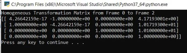
From the output, we can see that the displacement vector (upper right corner of the homogeneous transformation matrix) is x = 4 cm, y = 10 cm, and z = 10 cm.

Now that we have simulated our two degree of freedom robotic arm, let’s work with a real robot.

Working With a Real Robot

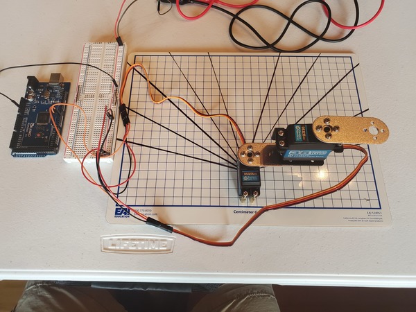
Let’s work with a real two degree of freedom robot to see if what we get on the real robot agrees with our derivation of the homogeneous transformation matrix in the previous section.

Write the Arduino Code

We want the robot to move from the starting position (as noted in the kinematic diagram) to the following joint angles:

servo_0_angle = 45 degrees # Joint 1 (θ₁)
servo_1_angle = 45 degrees # Joint 2 (θ₂)

Here is the code. Note that for servo 1, the range is from -90 to 90 degrees, so we need to map that value to an equivalent servo value between 0 and 180 degrees.
The name of the program is 2dof_robotic_arm_45_degrees.ino:

/*
Program: Move Servos on 2DOF Robot to 45 Degrees Using Arduino
File: 2dof_robotic_arm_45_degrees.ino
Description: This program sweeps two servos (i.e. joints) from 0 degrees to 45 degrees.
  Note that Servo 0 = Joint 1 and Servo 1 = Joint 2.
Author: Addison Sears-Collins
Website: https://automaticaddison.com
Date: August 23, 2020
*/
 
#include <VarSpeedServo.h> 

// Define the number of servos
#define SERVOS 2

// Create the servo objects.
VarSpeedServo myservo[SERVOS]; 

// Speed of the servo motors
// Speed=1: Slowest
// Speed=255: Fastest.
const int desired_speed = 75;

// Desired Angle in degrees
const int desired_servo_angle = 45;

// Attach servos to digital pins on the Arduino
int servo_pins[SERVOS] = {3,5};

void setup() {
  
  // Attach the servos to the servo object 
  // attach(pin, min, max  ) - Attaches to a pin 
  //   setting min and max values in microseconds
  //   default min is 544, max is 2400  
  // Alter these numbers until both servos have a 
  //   180 degree range.
  myservo[0].attach(servo_pins[0], 544, 2475);  
  myservo[1].attach(servo_pins[1], 500, 2475); 

  // Set initial servo positions 
  myservo[0].write(0, desired_speed, true);  
  myservo[1].write(calc_servo_1_angle(0), desired_speed, true);

  // Wait one second to let servos get into position
  delay(1000);
}
 
void loop() {  

    // Go to 45 degrees
    myservo[0].write(desired_servo_angle, desired_speed, true); 

    // Go to 45 degrees
    myservo[1].write(calc_servo_1_angle(desired_servo_angle), desired_speed, true); 
    
    // Wait half a second
    delay(500);
}     

/*  This method converts the desired angle for Servo 1 into a control angle
 *  for Servo 1. It assumes that the 0 degree position on the kinematic
 *  diagram for Servo 1 is actually 90 degrees on the actual servo.
 *  The angle range for Servo 1 on the kinematic diagram is
 *  -90 to 90 degrees, with 0 degrees being the center position. 
 *  The actual servo range for the physical motor
 *  is 0 to 180 degrees. We convert the desired angle 
 *  to a value within that range.
 */
int calc_servo_1_angle (int input_angle) {
  
  int result;

  result = map(input_angle, -90, 90, 0, 180);

  return result;
}

Run the Code

Upload your code to your Arduino board and run the code. Here is what you should see:

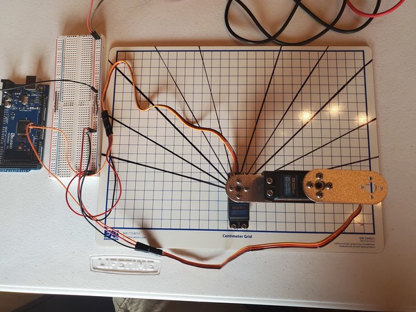
Mark the Position of the End Effector

Take a dry erase marker and mark the end of the end effector on the dry erase board.

The marker should have marked the dry erase board near the coordinate (x=4, y=10).

This result should agree with the Python code we wrote earlier in this tutorial.

References

Credit to Professor Angela Sodemann from whom I learned these important robotics fundamentals. Dr. Sodemann teaches robotics over at her website, RoboGrok.com. While she uses the PSoC in her work, I use Arduino and Raspberry Pi since I’m more comfortable with these computing platforms. Angela is an excellent teacher and does a fantastic job explaining various robotics topics over on her YouTube channel.