
In this section, we’ll learn how to find the Denavit-Hartenberg Parameter table for robotic arms. This method is a shortcut for finding homogeneous transformation matrices and is commonly seen in documentation for industrial robots as well as in the research literature. The real-world example we’ll consider in this tutorial is a SCARA robotic arm, like the one below.
Remember that homogeneous transformation matrices enable you to express the position and orientation of the end effector frame (e.g. robotics gripper, hand, vacuum suction cup, etc.) in terms of the base frame.
To calculate the homogeneous transformation matrix from the base frame to the end effector frame, the only values you need to have are the length of each link and the angle of each servo motor.
The Three Steps
Here are the three steps for finding the Denavit-Hartenbeg parameter table and the homogeneous transformation matrices for a robotic manipulator:
1. Draw the kinematic diagram according to the four Denavit-Hartenberg rules.
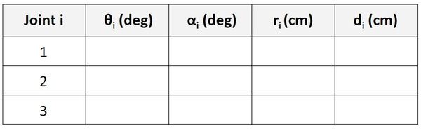
2. Create the Denavit-Hartenberg parameter table.
- Number of Rows = Number of Frames – 1
- Number of Columns = 4: Two columns for rotation and two columns for displacement
3. Find the homogeneous transformation matrices (I’ll cover how to do this step in my next post).
Definition of the Parameters
The Denavit-Hartenberg parameter tables consist of four variables:
- The two variables used for rotation are θ and α.
- The two variables used for displacement are r and d.
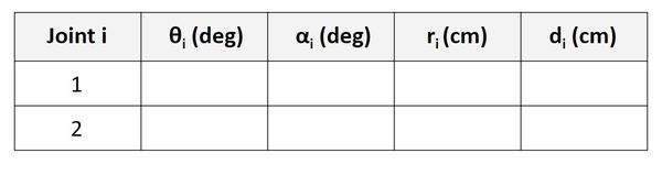
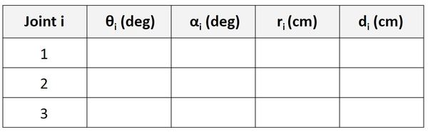
Here is the D-H parameter table template for a robotic arm with four reference frames:
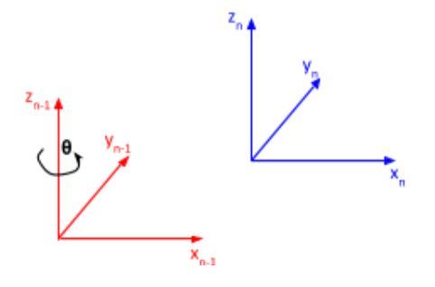
Let’s take a look at what these parameters mean by looking at two different frames. The n-1 frame is the frame before the n frame. We assume that both frames are connected by a link.
For example, if the n-1 frame is frame 2, the n frame is frame 3.
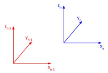
θ is the angle from xn-1 to xn around zn-1.
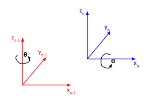
α is the angle from zn-1 to zn around xn.
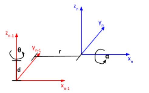
r (sometimes you’ll see the letter ‘a’ instead of ‘r’) is the distance between the origin of the n-1 frame and the origin of the n frame along the xn direction.
d is the distance from xn-1 to xn along the zn-1 direction.
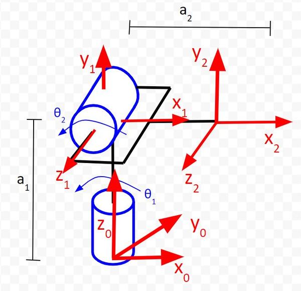
Example 1 – Two Degree of Freedom Robotic Arm
Let’s take a look at an example so that we can walk through the process of creating and filling in Denavit-Hartenberg parameter tables.
Draw the Kinematic Diagram According to the Denavit-Hartenberg Rules
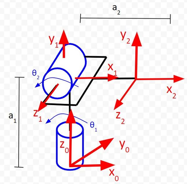
We’ll start by drawing the kinematic diagram of a two degree of freedom robotic arm.
Create the Denavit-Hartenberg Parameter Table
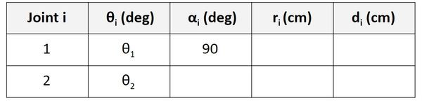
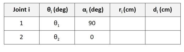
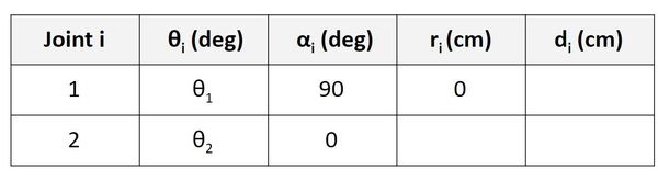
Now, we need to find the Denavit-Hartenberg parameters. We have three coordinate frames here, so we need to have two rows in our D-H table (i.e. number of rows = number of frames – 1).
Find θ
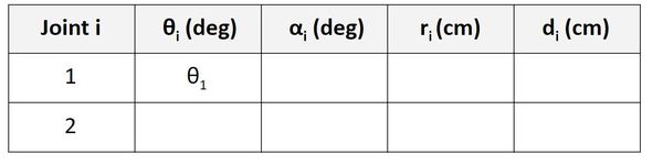
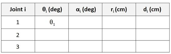
For the Joint 1 (Servo 0) row, we are going to focus on the relationship between frame 0 and frame 1. θ is the angle from x0 to x1 around z0.
If you look at the diagram, x0 and x1 both point in the same direction. The axes are therefore aligned. When the robot is in motion, θ1 will change (which will cause frame 1 to move relative to frame 0). The angle from x0 to x1 around z0 will be θ1, so let’s put that in our table.
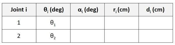
Now, let’s look at the Joint 2 (Servo 1) row. We take a look at the rotation between frame 1 and frame 2. θ is the angle from x1 to x2 around z1.
If you look at the diagram, x1 and x2 both point in the same direction. The axes are therefore aligned. When the robot is in motion, θ2 will change (which will cause frame 2 to move). The angle from x1 to x2 around z1 will be θ2, so let’s put that in the second row of our table.
Find α
Let’s start with the Joint 1 (Servo 0) row of the table.
α is the angle from z0 to z1 around x1.
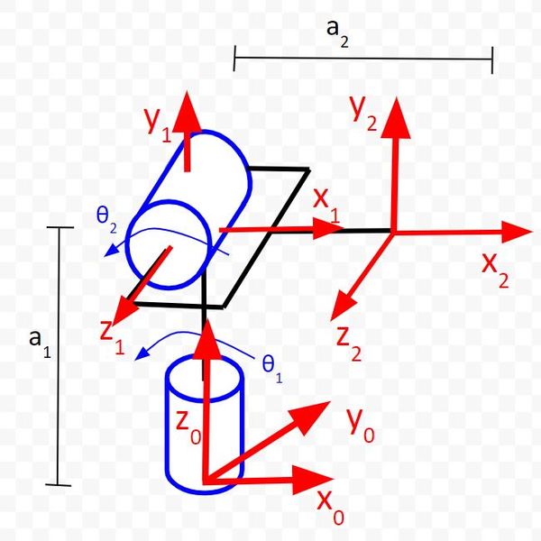
In the diagram above, you can see that this angle is 90 degrees, so we put 90 in the table.
Let’s go to the Joint 2 row of the table.
α is the angle from z1 to z2 around x2. You can see that no matter what happens to θ2, the angle from z1 to z2 will be 0 (since both axes point in the same direction). We put 0 degrees into the table.
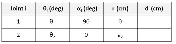
Find r
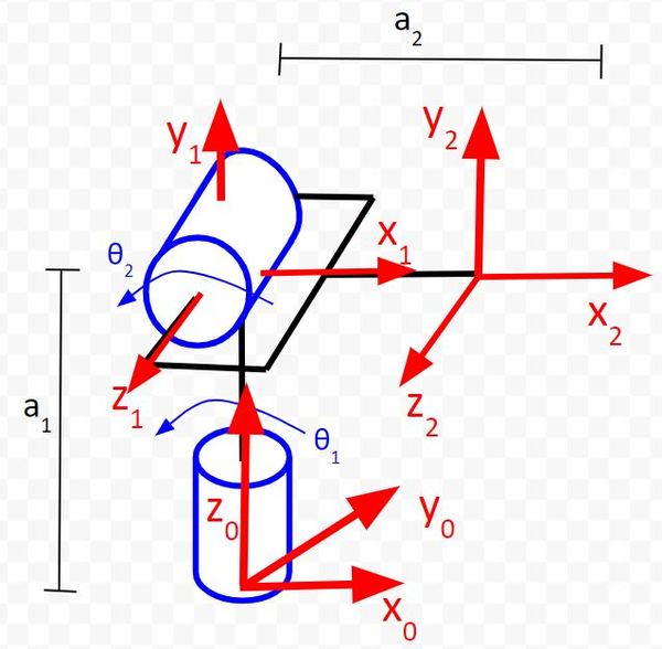
Let’s start with the Joint 1 row of the table.
r is the distance between the origin of frame 0 and the origin of frame 1 along the x1 direction. You can see in the diagram that this distance is 0.
Now let’s look at the Joint 2 row. r is the distance between the origin of frame 1 and the origin of frame 2 along the x2 direction. You can see in the diagram that this distance is a2.
Find d
Now let’s find d. We’ll start on the first row of the table as usual.
d is the distance from x0 to x1 along the z0 direction. You can see that this distance is a1.
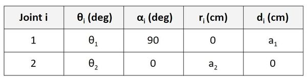
Now let’s take a look at frame 1 to frame 2. d is the distance from x1 to x2 along the z1 direction. You can see that this distance is 0.
Example 2 – SCARA Robot
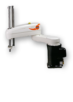
Let’s get some more practice filling in D-H parameter tables by looking at the SCARA robot.
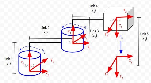
Draw the Kinematic Diagram According to the Denavit-Hartenberg Rules
Here is the kinematic diagram using the D-H convention.
Create the Denavit-Hartenberg Parameter Table
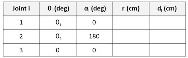
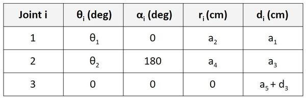
Now, we need to find the Denavit-Hartenberg parameters. We have four coordinate frames here, so we need to have three rows in our D-H table.
Find θ
For the Servo 0 row, we are going to focus on the relationship between frame 0 and frame 1. θ is the angle from x0 to x1 around z0.
If you look at the diagram, x0 and x1 both point in the same direction. The axes are therefore aligned. When the robot is in motion, θ1 will change (which will cause frame 1 to move). The angle from x0 to x1 around z0 will be θ1, so let’s put that in our table.
Now, let’s look at the Servo 1 row. We take a look at the rotation between frame 1 and frame 2. θ is the angle from x1 to x2 around z1.
If you look at the diagram, x1 and x2 both point in the same direction. The axes are therefore aligned. When the robot is in motion, θ2 will change (which will cause frame 2 to move). The angle from x1 to x2 around z1 will be θ2, so let’s put that in the second row of our table.
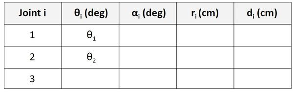
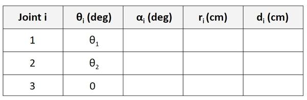
Now, let’s look at the Servo 2 row. We take a look at the rotation between frame 2 and frame 3. θ is the angle from x2 to x3 around z2.
If you look at the diagram, x2 and x3 both point in the same direction. The axes are therefore aligned. When the robot is in motion, there is only linear motion along z2. The angle from x2 to x3 around z2 will remain 0, so let’s put that in the third row of our table.
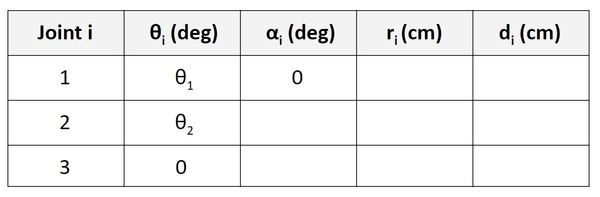
Find α
Let’s start with the Servo 0 row of the table.
α is the angle from z0 to z1 around x1.
In the diagram above, you can see that this angle is 0 degrees, so we put 0 in the table.
Let’s go to the Servo 1 row of the table.
α is the angle from z1 to z2 around x2. In the diagram above, you can see that this angle is 180 degrees, so we put 180 in the table.
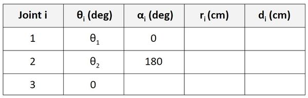
Let’s go to the Servo 2 row of the table.
α is the angle from z2 to z3 around x3. In the diagram above, you can see that this angle is 0 degrees, so we put 0 in the table.
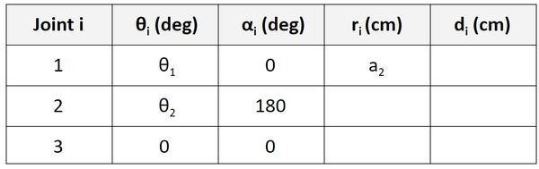
Find r
Let’s start with the Servo 0 row of the table.
r is the distance between the origin of frame 0 and the origin of frame 1 along the x1 direction. You can see in the diagram that this distance is a2.
Now let’s look at the Servo 1 row. r is the distance between the origin of frame 1 and the origin of frame 2 along the x2 direction. You can see in the diagram that this distance is a4.
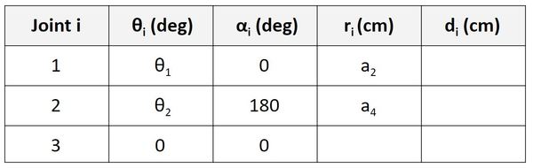
Now let’s look at the Servo 2 row. r is the distance between the origin of frame 2 and the origin of frame 3 along the x3 direction. You can see in the diagram that this distance is 0.
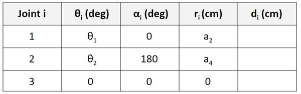
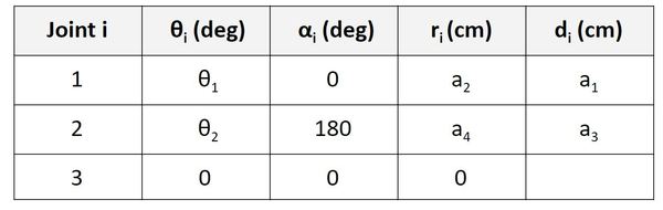
Find d
Now let’s find d. We’ll start on the first row of the table as usual.
d is the distance from x0 to x1 along the z0 direction. You can see that this distance is a1.
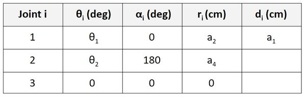
Now let’s take a look at frame 1 to frame 2. d is the distance from x1 to x2 along the z1 direction. You can see that this distance is a3.
Now let’s take a look at frame 2 to frame 3. d is the distance from x2 to x3 along the z2 direction. You can see that this distance is a5 + d3.
References
Credit to Professor Angela Sodemann for teaching me this stuff. She is an excellent teacher (She runs a course on RoboGrok.com). On her YouTube channel, she provides some of the clearest explanations on robotics fundamentals you’ll ever hear.