In this tutorial, we’ll learn about the Jacobian matrix, a useful mathematical tool for robotics.

Table of Contents

Real-World Applications

There are some use cases (e.g. robotic painting) where we want to control the velocity of the end effector (i.e. paint sprayer, robotic hand, gripper, etc.) of a robotic arm. One way to do this is to use a library to set the desired speed of each joint on a robotic arm. I did exactly this in this post.

1-Robotic-spray-painting-experiment — A car painting robot. If the robotic arms move too fast, they will do a poor job painting the vehicle. We can use Jacobian matrices to help control the speed of the arm. Image Source: ResearchGate.

Another way we can do this is to use a mathematical tool called the Jacobian matrix. The Jacobian matrix helps you convert angular velocities of the joints (i.e. joint velocities) into the velocity of the end effector of a robotic arm.

For example, if the servo motors of a robotic arm are rotating at some velocity (e.g. in radians per second), we can use the Jacobian matrix to calculate how fast the end effector of a robotic arm is moving (both linear velocity x, y, z and angular velocity roll ω_x, pitch ω_y, and yaw ω_z).

Prerequisites

It is helpful if you know how to do the following:

Overview of the Jacobian Matrix

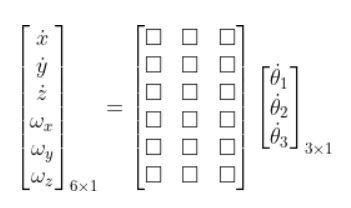
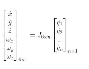
For a robot that operates in three dimensions, the Jacobian matrix transforms joint velocities into end effector velocities using the following equation:

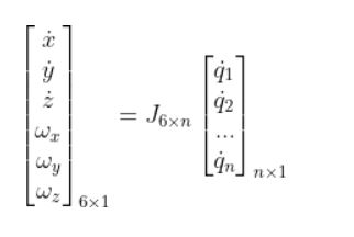
q with the dot on top represents the joint velocities (i.e. how fast the joint is rotating for a revolute joint and how fast the joint is extending or contracting for a prismatic joint) .

The size of this vector is n x 1, with n being equal to the number of joints (i.e. servo motors or linear actuators) in your robotic arm.
Note that q can represent either revolute joints (typically represented as θ) or prismatic joints (which I usually represent as d, which means displacement)

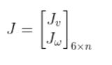
J is the Jacobian matrix. It is an m rows x n column matrix (m=3 for two dimensions, and m=6 for a robot that operates in three dimensions). n represents the number of joints.

The matrix on the left represents the velocities of the end effector.

x, y, and z with the dots on top represent linear velocities (i.e. how fast the end effector is moving in the x, y, and z directions relative to the base frame of a robotic arm)

ω_x, ω_y, and ω_zrepresent the angular velocities (i.e. how fast the end effector is rotating around the x, y, and z axis of the base frame of a robotic arm).

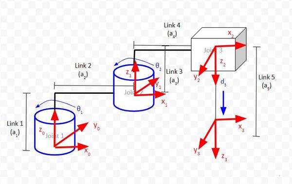
Consider this SCARA robotic arm:

The equation using the Jacobian would be as follows:

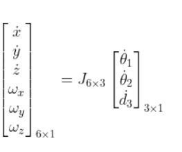
Looking closer at the Jacobian, this term can be divided into two parts, where the first three rows are used for linear velocities, and the bottom three rows are used for angular velocities.

Taking a look at a real-world example, you’ll see that the SCARA robot that I’ve been building (see my YouTube video here) can only rotate around the z axis of the base frame (i.e. straight upwards towards the ceiling out of the board). There is no rotation around the x or y axes of the base frame.

How To Find the Jacobian Matrix for a Robotic Arm

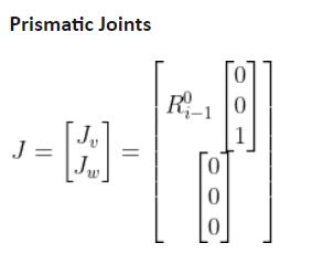
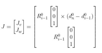
To fill in the Jacobian matrix, we use the following tables:

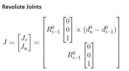
The upper half of the matrix is used to determine the linear components of the velocity, while the bottom part is used to determine the rotational components of the velocity.

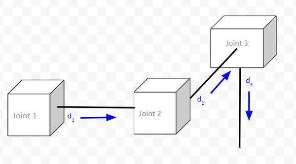
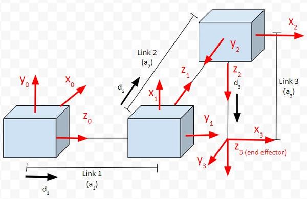
Example 1: Cartesian Robot

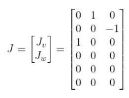
Consider the following robot that has three prismatic joints.

Here is the equation with the Jacobian matrix:

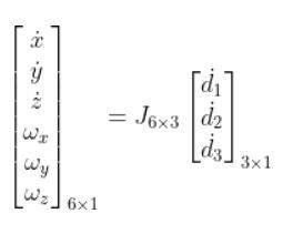
Which is the same as:

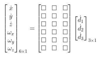
Notice that the q’s were replaced with d’s, which represent “displacement” of the prismatic joint (i.e. linear actuator).

To fill in the Jacobian matrix, we have to come one column at a time from left to right. Each column represents a single joint.

Let’s start with Joint 1. Making i = 1, we get:

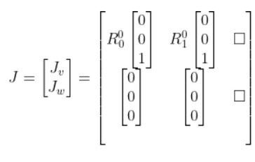
Now let’s fill in the second column of the matrix which represents Joint 2. Making i = 2, we get:

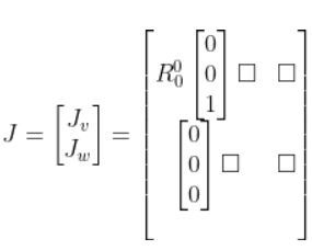
Finally, let’s fill in column 3, which represents Joint 3.

The R in the matrix above stands for “rotation matrix.” For example, R⁰₁stands for the rotation matrix from frame 0 to frame 1.

Now to fill in the rotation matrices, we need to add reference frames to the joints. This tutorial shows you how to do that. I’m going to use that same graphic here.

Let’s start with R⁰₀. Since we have no rotation from frame to frame 0, R⁰₀is the identity matrix. Anything that is multiplied by the identity matrix will remain itself, so our matrix now looks like this:

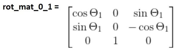
What is R⁰₁? We derived this matrix here.

So now we have:

Which reduces to:

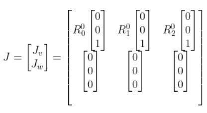
What is R⁰₂? We know that:

R⁰_{2 =}R⁰₁R¹₂

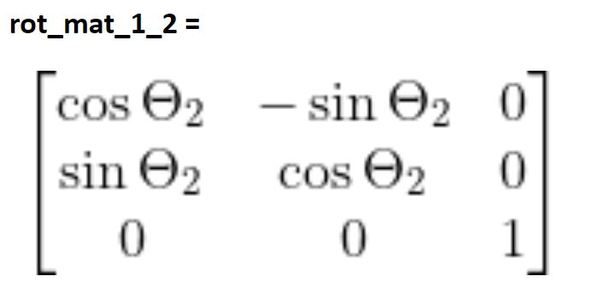
Here is R¹₂:

Therefore:

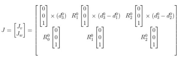
Our Jacobian becomes:

Which reduces to:

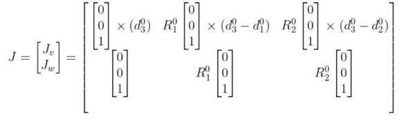
Writing this a bit more clearly, we have:

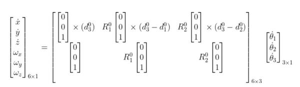
Our original equation then becomes:

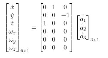
We can do matrix multiplication on the right side of this equation above to yield six equations:

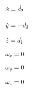
If we look at the kinematic diagram, we can see if the equations above make sense. You can see that the speed of the end effector in the x₀direction is determined by the displacement of joint 2 (i.e. d₂).

You can see that the speed of the end effector in the y₀direction is determined by the negative displacement of joint 3 (i.e. d₃).

The speed of the end effector in the z₀direction is determined by the positive displacement of joint 1 (i.e. d₁).

The last three equations tell us that the end effector will never be able to rotate around the x, y, and z axes of frame 0, the base frame of the robot. This makes sense because all of the joints are prismatic joints. We would need to have revolute joints in order to get rotation.

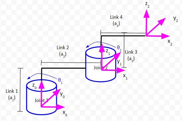
Example 2: Articulated Robot

Now let’s take a look at another example, an articulated robot that has the following kinematic diagram.

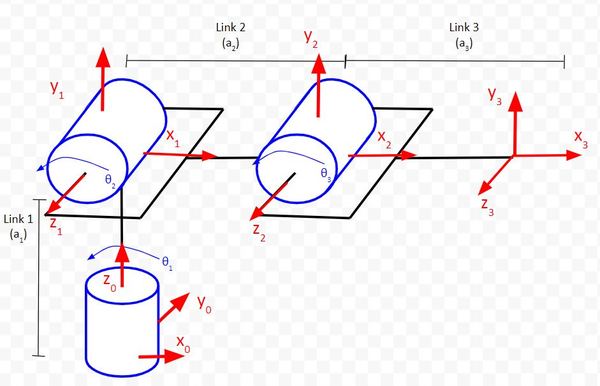
This robotic arm will have three columns since it has three joints (i.e. servo motors). As usual, it will have six rows since we’re working in three dimensions.

Our equation that relates joint velocity to the velocity of the end effector takes the following form:

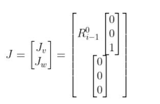
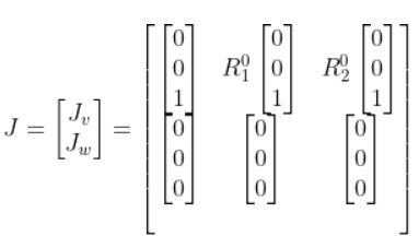
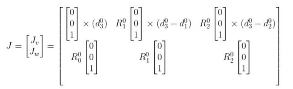
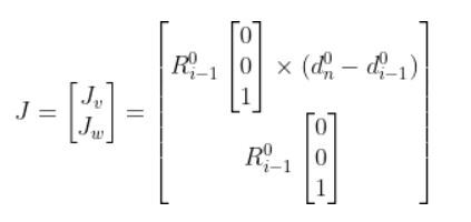
The Jacobian matrix J (the 6×3 matrix above with the squares) takes the following form since we have all revolute joints:

So using the form above, our Jacobian matrix for the articulated robotic arm is (n is the number of joints):

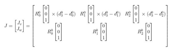
You’ll see that each column (i = 1, 2, and 3) uses the Jacobian for revolute joints since each joint is a revolute joint.

The x in the above matrix stands for the cross product.

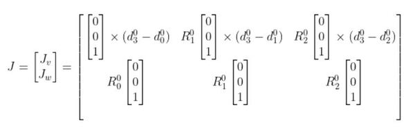
Now, let’s fill in this Jacobian matrix, going one column at a time from left to right.

R⁰₀ is the identity matrix since there is no rotation from frame 0 to itself.

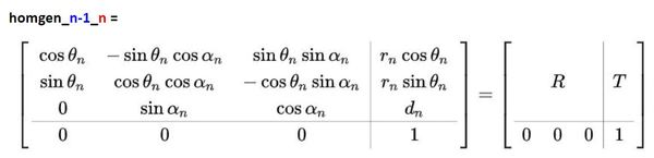
We now need to find d⁰₃. d⁰₃comes from the upper right of the homogeneous transformation matrix from frame 0 to frame 3 (i.e. homgen_0_3). That is, it comes from the T part of the matrix of the following form:

To get the homogeneous transformation matrix from frame 0 to frame 3, we first have to fill in the Denavit-Hartenberg table for the articulated robotic arm. I show you how to do this in this tutorial.

Here was the table we got:

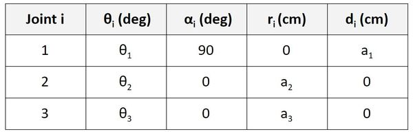
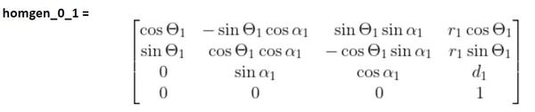
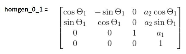
Now, we take a look at that table and go one row at a time, starting with the Joint 1 row. To find the homogeneous transformation matrix from frame 0 to frame 1, we use the values from the first row of the table to fill in this…

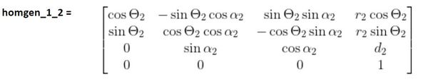
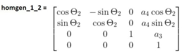
We then look at the second row of the D-H table and fill in the homogeneous transformation matrix from frame 1 to 2…

We then look at the third row of the D-H parameter table to fill in the homogeneous transformation matrix from frame 2 to 3…

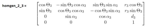
Then, to find the homogeneous transformation matrix from the base frame (frame 0) to the end-effector frame (frame 3), we would multiply those three transformation matrices together.

homgen_0_3 = (homgen_0_1)(homgen_1_2)(homgen_2_3)

d⁰₃is a three element vector that is made up of the values of the first three rows of the rightmost column of homgen_0_3. I won’t go through all the matrix multiplication for finding homgen_0_3, but if you follow the method I’ve described above, you will be able to get it.

d⁰₀will always be 0, so our Jacobian will look like this at this stage:

Going to the second column of the matrix, d⁰₁is a three element vector that is made up of the values of the first three rows of the rightmost column of homgen_0_1 (which you found earlier).

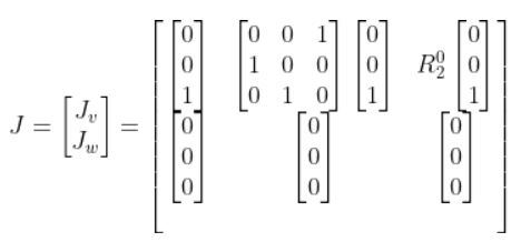
R⁰₁is below (see this tutorial for how to find it):

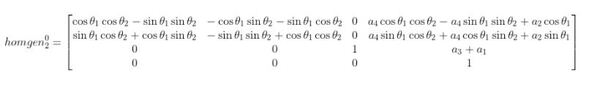
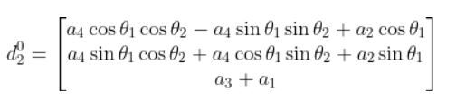
Going to the third column, d⁰₂is a three element vector that is made up of the values of the first three rows of the rightmost column of homgen_0_2. Since you know homgen_0_1 and homgen_1_2, you can multiply those two matrices together to get homgen_0_2.

homgen_0_2 = (homgen_0_1)(homgen_1_2)

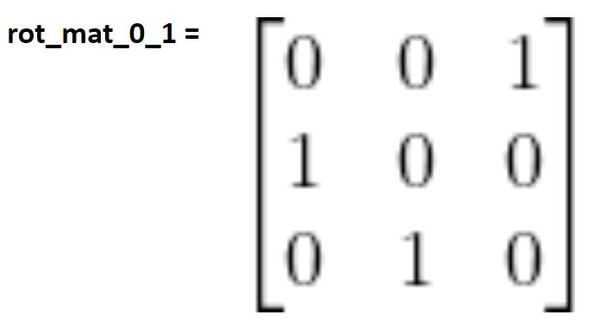
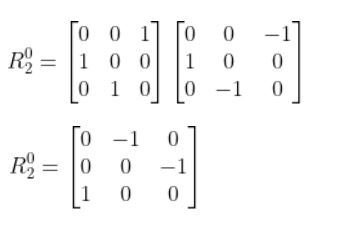
R⁰₂(i.e. rot_mat_0_2) is found by multiplying the rotation matrices from frame 0 to frame 1 and from frame 1 to frame 2.

rot_mat_0_2 = (rot_mat_0_1)(rot_mat_1_2)

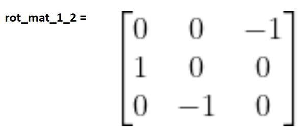
We know rot_mat_0_1. Rot_mat_1_2 is the following:

Now in the top half your Jacobian matrix you will need to go column by column and take the cross product of two three-element vectors.

In a real-world setting, you would use a Python library like NumPy to perform this operation. If you do a search for “numpy.cross” you will see how to do this. For example, here is some Python code of how to take the cross product of two three-element vectors:

x = [1, 2, 3]
y = [4, 5, 6]
np.cross(x, y)
Output:
array([-3,  6, -3])

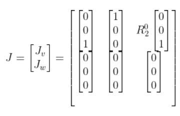
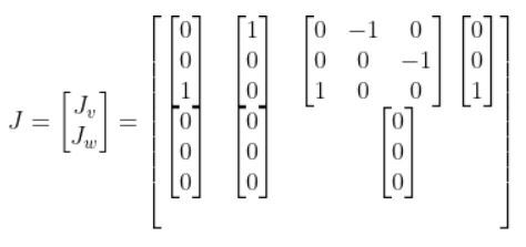
Now going to the bottom half of the matrix, R⁰₀ is the identity matrix.

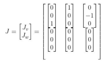
You can fill in the rest of the bottom half of the Jacobian matrix because we know R⁰₁ and R⁰₂.

Once you have the Jacobian, you will then have the following setup:

From the setup above, you can find six equations, one for each velocity variable (on the far left). These equations enable us to calculate the velocities of the end effector of the articulated robotic arm given the joint velocities.

Inverse Jacobian Matrix

In the previous section, we looked at how to calculate the velocities of the end effector of a robotic arm given the joint velocities. What if we want to do the reverse? We want to calculate the joint velocities given desired velocities of the end effector?

To solve this problem, we must use the inverse of the Jacobian matrix.

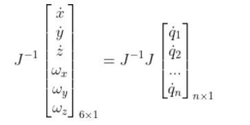
A matrix multiplied by its inverse is the identity matrix I. The identity matrix is the matrix version of the number 1.

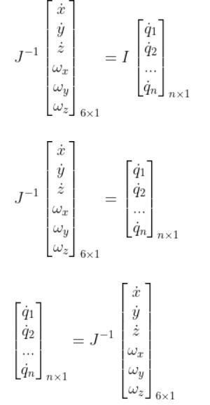
You can only take the inverse of a square matrix. A square matrix is a matrix where the number of rows is equal to the number of columns.

So how would we find J^-1? Let’s take a look at an example.

Example

Suppose we have the following two degrees of freedom robotic arm.

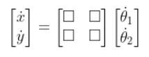
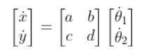
We have the following equation where the matrix with the 12 squares is J, the Jacobian matrix.

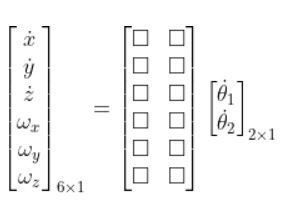
We only have two servo motors. These two servo motors control the velocity of the end effector in only the x and y directions (e.g. we have no motion in the z direction).

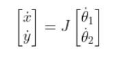
Suppose the only thing that matters to us is the linear velocity in the x direction and the linear velocity in the y direction. We can simplify our equation accordingly to this, where the matrix with the squares is J:

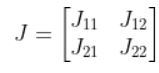
Let’s replace those squares with some variables.

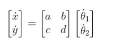
Since…

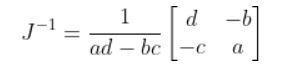
To get the J^-1, we use the following formula:

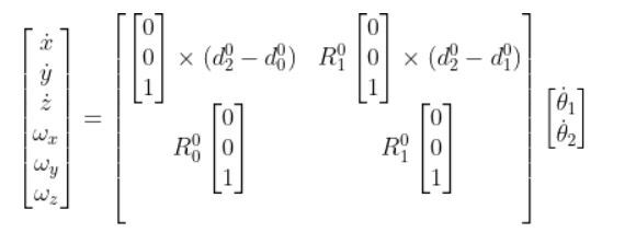
To get J^-1, we first need to find J. J has two revolute joints. Revolute joints take the following form:

So the equation for our two degree of freedom robotic arm will look like this:

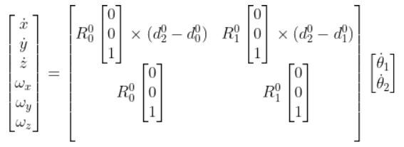
R⁰₀is the identity matrix.

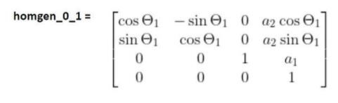
To calculate d⁰₂, we need to find the homogeneous transformation matrix from frame 0 to frame 2. We did exactly this on this tutorial.

homgen_0_2 = (homgen_0_1)(homgen_1_2)

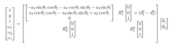
When you do this multiplication, you get the following:

Based on the homogeneous matrix above, here is d⁰₂.

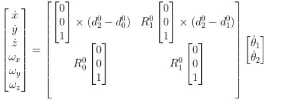
Plugging that into this expression below and performing the cross product with the vector [0 0 1], we get:

And since:

We know that:

R⁰₁ is the 3×3 matrix in the upper left of homgen_0_1.
d⁰₁is the 3×1 vector in the upper right of homgen_0_1.
We already know d⁰₂. We found that earlier in this tutorial.
We can therefore fill in the rest of the upper half of the Jacobian matrix to get this:

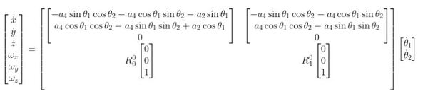
J is that big matrix above. Since we are only concerned about the linear velocities in the x and y directions, this:

Becomes…

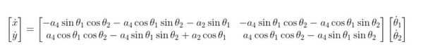
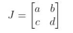
J is that big matrix above. It takes the form:

To get the inverse of J (i.e. J^-1), we do the following:

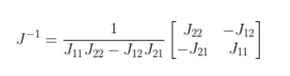
The (J₁₁J₂₂ – J₁₂J₂₁) in the denominator is known as the determinant. I’ll call 1/(J₁₁J₂₂ – J₁₂J₂₁) the reciprocal of the determinant.

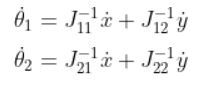
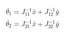
Once we know J^-1, we can use the following expression to solve the joint velocities given the velocities of the end effector in the x and y directions.

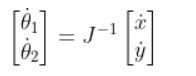
Which is the same as:

Which is:

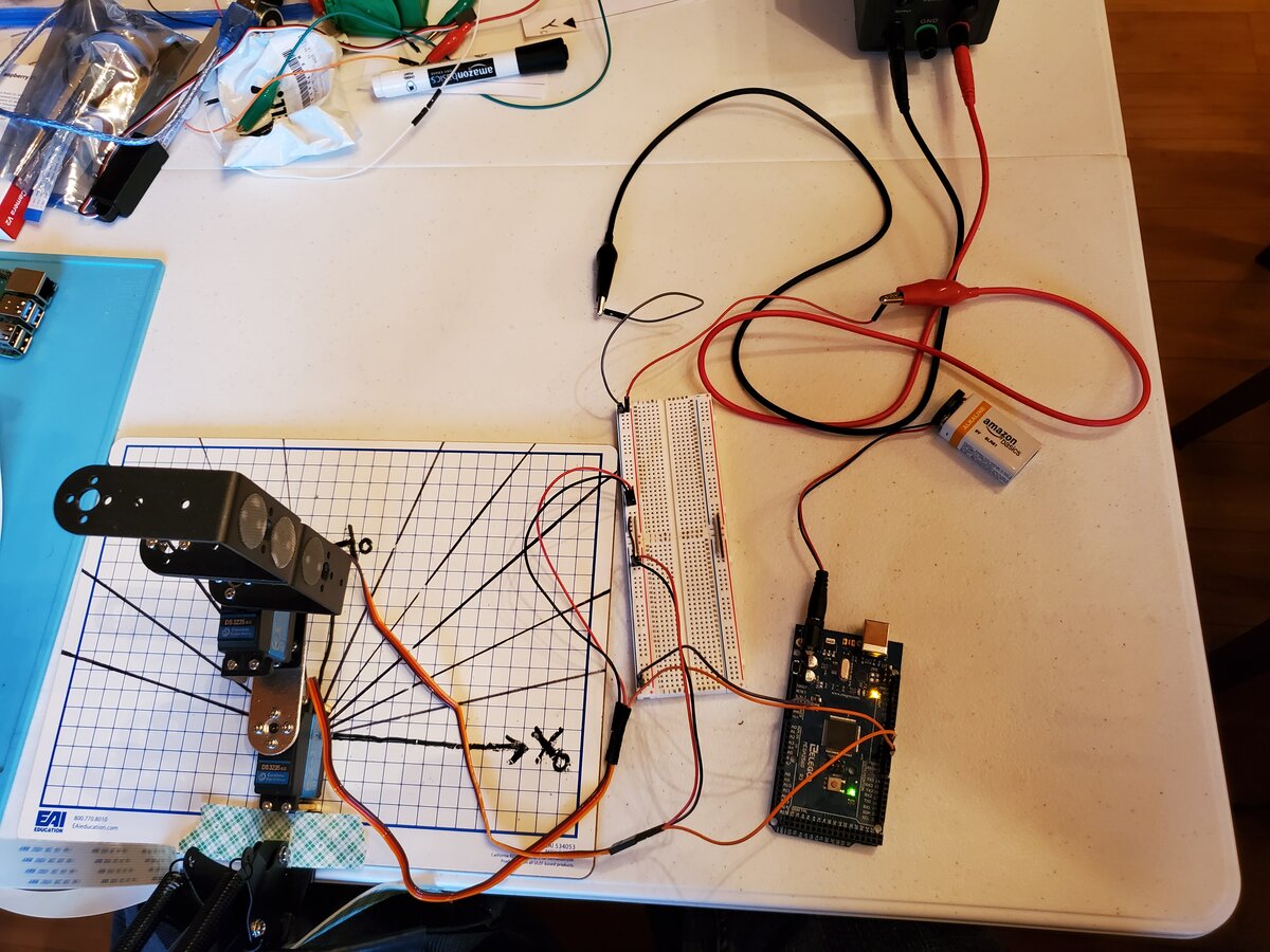
Programming the Jacobian on a Real Robot

Let’s take a look at all this math we’ve done so far by implementing it on a real-world robot.

To do this section, you need to have assembled the two degrees of freedom SCARA robot here.

We want to calculate the rotation velocity of the two joints (i.e. servo motors) based on desired linear velocities of the end effector.

We will program our robotic arm so that the end effector of the robotic arm moves in a straight line at a constant linear velocity.

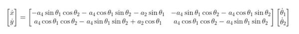
This equation will come in handy. That big nasty matrix below is the Jacobian. We’ll use it to calculate the inverse Jacobian matrix in our code.

Open the Arduino IDE and create a new sketch named jacobian_based_path_planning_v2.ino.

Write the following code. It is helpful to write the code line by line rather than copying and pasting so that you understand what is going on.

/*
Program: Jacobian-Based Path Planning
File: jacobian_based_path_planning_v1.ino
Description: This program moves the end effector of a SCARA robotic arm based on your
  desired x and y linear velocities. 
  Motion is calculated using the Jacobian matrix which relates joint velocities
  to end effector velocities.
  Note that Servo 0 = Joint 1 and Servo 1 = Joint 2.
Author: Addison Sears-Collins
Website: https://automaticaddison.com
Date: October 14, 2020
*/
 
#include <VarSpeedServo.h> 

// Define the number of servos
#define SERVOS 2

// Conversion factor from degrees to radians
#define DEG_TO_RAD 0.017453292519943295769236907684886

// Conversion factor from radians to degrees
#define RAD_TO_DEG 57.295779513082320876798154814105

// Create the servo objects.
VarSpeedServo myservo[SERVOS]; 

// Speed of the servo motors
// Speed=1: Slowest
// Speed=255: Fastest.
const int default_speed = 255;

const int std_delay = 10; // Delay in milliseconds

// Attach servos to digital pins on the Arduino
int servo_pins[SERVOS] = {3,5};

// Angle of the first servo
float theta_1 = 0;
float theta_1_increment = 0; 
float theta_1_dot = 0; // rotational velocity of the first servo

// Angle of the second servo
float theta_2 = 0;
float theta_2_increment = 0;
float theta_2_dot = 0; // rotational velocity of the second servo

// Linear velocities of the end effector relative to the base frame
// Units are in centimeters per second
// If x_dot = 0.0, the end effector will move parallel to the y axis
// Play around with these numbers, and observe the motion of the end effector
// relative to the x and y axes of the base frame of the robotic arm.
float x_dot = 0.0;
float y_dot = 1.0;

// Jacobian variables
float reciprocal_of_the_determinant;
float J11;
float J12;
float J21;
float J22;

// Inverse Jacobian variables
float J11_inv;
float J12_inv;
float J21_inv;
float J22_inv;

// Link lengths in centimeters
// You measure these values using a ruler and the kinematic diagram
float a2 = 5.9;
float a4 = 6.0;

void setup() {

  Serial.begin(9600);
  
  // Attach the servos to the servo object 
  // attach(pin, min, max  ) - Attaches to a pin 
  //   setting min and max values in microseconds
  //   default min is 544, max is 2400  
  // Alter these numbers until both servos have a 
  //   180 degree range.
  myservo[0].attach(servo_pins[0], 544, 2475);  
  myservo[1].attach(servo_pins[1], 500, 2475); 

  // Set the angle of the first servo.
  theta_1 = 0.0;

  // Set the angle of the second servo.
  theta_2 = 90.0;
  
  // Set initial servo positions 
  myservo[0].write(theta_1, default_speed, true);  
  myservo[1].write(theta_2, default_speed, true);

  // Let servos get into position
  delay(3000);
  
}
 
void loop() { 

    // Make sure the servos stay within their 180 degree range
    while (theta_1 <= 180.0 && theta_1 >= 0.0 && theta_2 <= 180.0 && theta_2 >= 0.0) { 

      // Convert from degrees to radians
      theta_1 = theta_1 * DEG_TO_RAD;
      theta_2 = theta_2 * DEG_TO_RAD;

      // Calculate the values of the Jacobian matrix
      J11 = -a4 * sin(theta_1) * cos(theta_2) - a4 * cos(theta_1) * sin(theta_2) - a2 * sin(theta_1);
      J12 = -a4 * sin(theta_1) * cos(theta_2) - a4 * cos(theta_1) * sin(theta_2);
      J21 = a4 * cos(theta_1) * cos(theta_2) - a4 * sin(theta_1) * sin(theta_2) + a2 * cos(theta_1);
      J22 = a4 * cos(theta_1) * cos(theta_2) - a4 * sin(theta_1) * sin(theta_2);
       
      reciprocal_of_the_determinant = 1.0/((J11 * J22) - (J12 * J21));

      // Calculate the values of the inverse Jacobian matrix
      J11_inv = reciprocal_of_the_determinant * (J22);
      J12_inv = reciprocal_of_the_determinant * (-J12);
      J21_inv = reciprocal_of_the_determinant * (-J21);      
      J22_inv = reciprocal_of_the_determinant * (J11);
      
      // Set the rotational velocity of the first servo
      theta_1_dot = J11_inv * x_dot + J12_inv * y_dot; 

      // Set the rotational velocity of the second servo
      theta_2_dot = J21_inv * x_dot + J22_inv * y_dot; 

      // Convert rotational velocity in radians per second to X radians in std_delay milliseconds
      // Note that 1 second = 1000 milliseconds and each delay is std_delay milliseconds
      theta_1_increment = (theta_1_dot) * (1/1000.0) * std_delay;

      // Convert rotational velocity in radians per second to X radians in std_delay milliseconds
      // Note that 1 second = 1000 milliseconds and each delay is std_delay milliseconds
      theta_2_increment = (theta_2_dot) * (1/1000.0) * std_delay;

      theta_1 = theta_1 + theta_1_increment; 
      theta_2 = theta_2 + theta_2_increment;

      // Convert the new angles from radians to degrees
      theta_1 = theta_1 * RAD_TO_DEG;
      theta_2 = theta_2 * RAD_TO_DEG;

      Serial.println(theta_1);
      Serial.println(theta_2);
      Serial.println(" ");
     
      myservo[0].write(theta_1, default_speed, true); 
      myservo[1].write(theta_2, default_speed, true);
      
      delay(std_delay); // Delay in milliseconds      
    }    
}

Load the code to your Arduino.

Wire up your system as shown on this pdf.

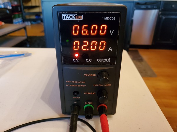
Set the voltage limit on your DC power supply to 6V and the current limit to 2A.

Run the code. You should see the end effector of your robotic arm move parallel to the y axis in a straight line because we set:

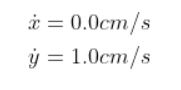
After a few seconds, the robotic arm will stop moving in a straight line. The reason for this is that the robotic arm can only move a fixed distance in the positive y direction due to the lengths of the links. The servos, however, continue to rotate until either the first servo or the second servo (or both) reach the limit of their range of rotation (i.e. 0 to 180 degrees).

That’s it! Keep building!

References

Sodemann, Dr. Angela 2020, RoboGrok, accessed 14 October 2020, <http://robogrok.com/>