
Inverse kinematics is about calculating the angles of joints (i.e. angles of the servo motors on a robotic arm) that will cause the end effector of a robotic arm (e.g. robotics gripper, hand, vacuum suction cup, etc.) to reach some desired position (x, y, z) in 3D space.
In this tutorial, we will learn about how to perform inverse kinematics for a six degree of freedom robotic arm. We will build from the work we did on this post where we used the graphical approach to inverse kinematics for a two degree of freedom SCARA-like robotic arm. This approach is also known as the analytical approach. It involves a lot of trigonometry and is fine for a robotic arm with three joints or less.
However, when we have a robotic arm with more than three degrees of freedom, we have to modify how we solve the inverse kinematics.
In this tutorial, we’ll take a look at two approaches: an analytical approach and a numerical approach. We’ll then code these up in Python so that you can see how the calculations are done in actual code.
Real-World Applications
- This post contains a list of a lot of the applications of six degree of freedom robotic arms.
Prerequisites
Analytical Approach vs Numerical Approach to Inverse Kinematics
The analytical approach to inverse kinematics involves a lot of matrix algebra and trigonometry.
The advantage of this approach is that once you’ve drawn the kinematic diagram and derived the equations, computation is fast (compared to the numerical approach, which is iterative). You don’t have to make initial guesses for the joint angles like you do in the numerical approach (we’ll look at this approach later in this tutorial).
The disadvantage of the analytical approach is that the kinematic diagram and trigonometric equations are tedious to derive. Also, the solutions from one robotic arm don’t generalize to other robotic arms. You have to derive new equations for each new robotic arm you work with that has a different kinematic structure.
Analytical Approach to Inverse Kinematics
In this section, we’ll explore one analytical approach to inverse kinematics (i.e. there are many approaches).
Assumptions
In this approach, we first need to start off by making some assumptions.
We have to assume that:
- The first three joints of the robotic arm are the only ones that determine the position of the end effector.
- The last three joints (and any other joints after that) determine the orientation of the end effector.
Overall Steps
Here are the steps for calculating inverse kinematics for a six degree of freedom robotic arm.
Step 1: Draw the kinematic diagram of just the first three joints, and perform inverse kinematics using the graphical approach.
Step 2: Compute the forward kinematics on the first three joints to get the rotation of joint 3 relative to the global (i.e. base) coordinate frame. The outcome of this step will yield a matrix rot_mat_0_3, which means the rotation of frame 3 relative to frame 0 (i.e. the global coordinate frame).
Step 3: Calculate the inverse of rot_mat_0_3.
Step 4: Compute the forward kinematics on the last three joints, and extract the part that governs the rotation. This rotation matrix will be denoted as rot_mat_3_6.
Step 5: Determine the rotation matrix from frame 0 to 6 (i.e. rot_mat_0_6).
Step 6: Taking our desired x, y, and z coordinates as input, use the inverse kinematics equations from Step 1 to calculate the angles for the first three joints.
Step 7: Given the joint angles from Step 6, use the rotation matrix to calculate the values for the last three joints of the robotic arm.
Let’s run through an example.
Draw the Kinematic Diagram of Just the First Three Joints and Do Inverse Kinematics
First, let’s draw the kinematic diagram for our entire robot. If you need a refresher on how to draw kinematic diagrams, check out this tutorial.
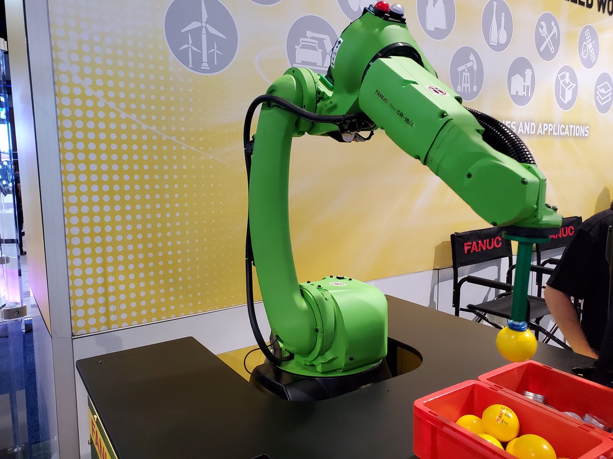
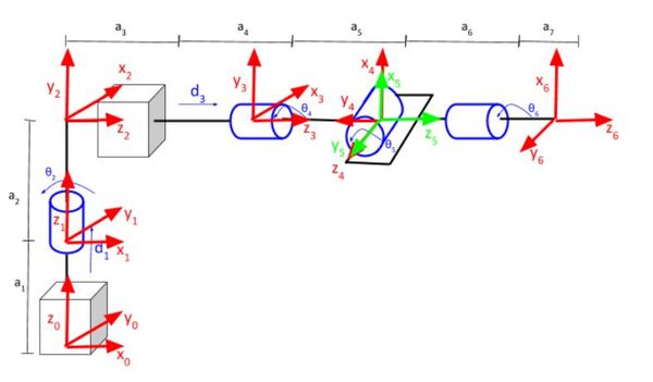
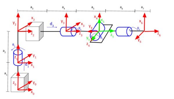
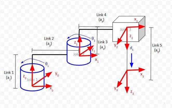
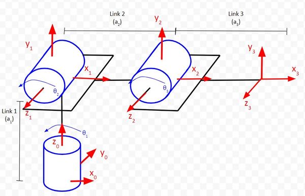
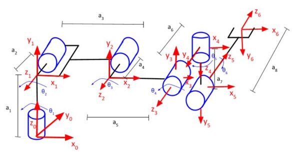
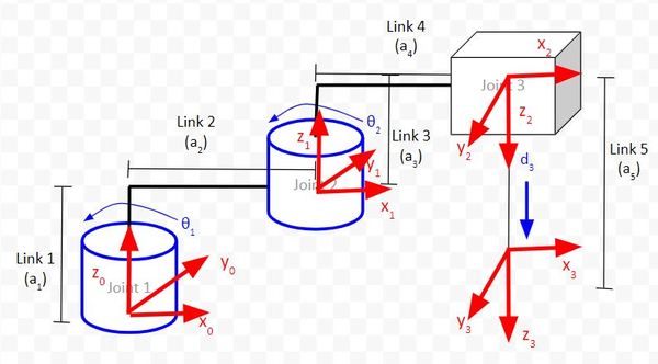
Our robotic arm will have a cylindrical-style base (i.e. range of motion resembles a cylinder) and a spherical wrist (i.e. range of motion resembles a sphere). Here is its kinematic diagram:
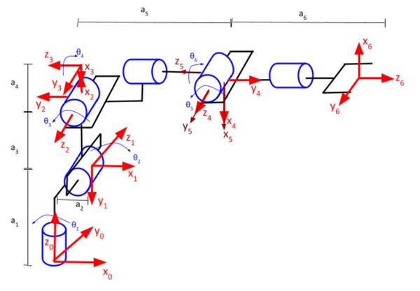
Here is the kinematic diagram of just the first three joints:
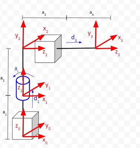
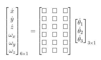
Let’s do inverse kinematics for the diagram above using the graphical approach to inverse kinematics. We first need to draw the aerial view of the diagram above.
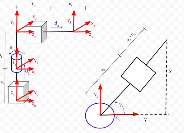
From the aerial view, we can see that we have two equations that come out of that.
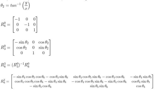
- θ2 = tan-1(y/x)
- d3 = sqrt(x2 + y2) – a3 – a4
Now, let’s draw the side view of the robotic arm (sorry for the tiny print).
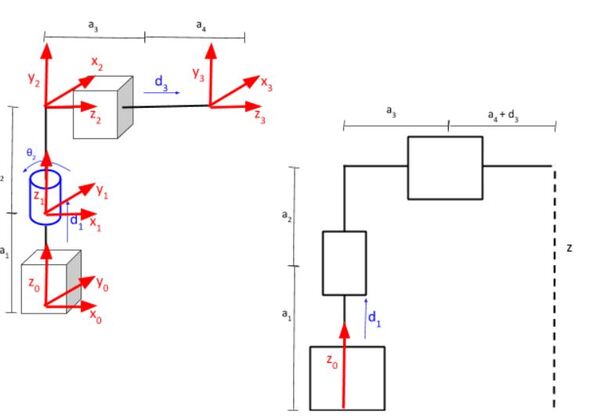
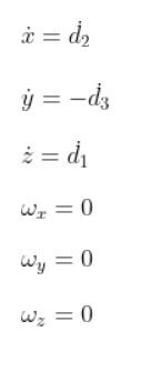
We can see from the above image that:
- d1 = z – a1 – a2
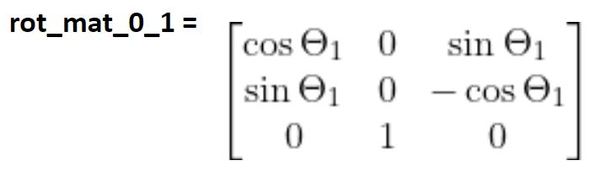
Calculate rot_mat_0_3
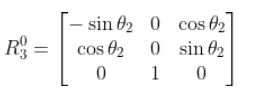
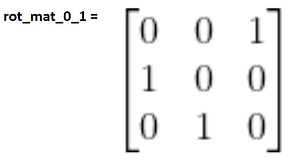
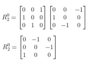
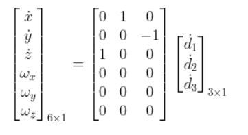
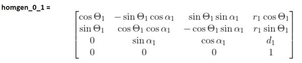
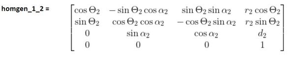
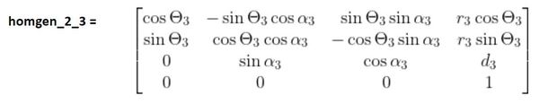
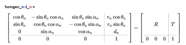
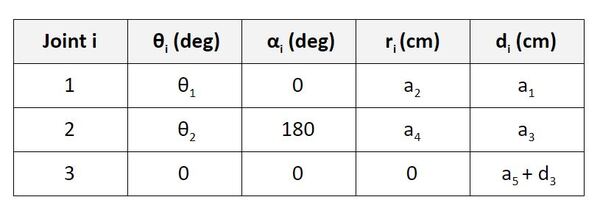
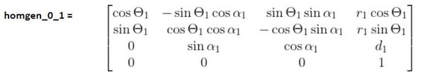
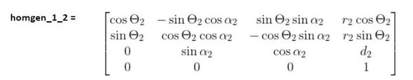
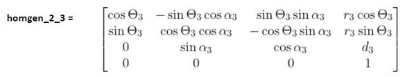
For this step, you can either use this method or the Denavit-Hartenberg method to calculate the rotation matrix of frame 3 relative to frame 0. Either of those methods will yield the following rotation matrix:
Calculate the Inverse of rot_mat_0_3
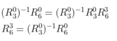
Now that we know rot_mat_0_3 (which we defined in the previous section), we need to take its inverse. The reason for this is due to the following expression:
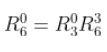
We can left-multiply the inverse of the rotation matrix we found in the previous section to solve for rot_mat_3_6.
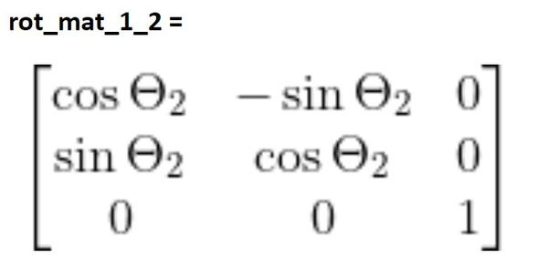
Calculate rot_mat_3_6
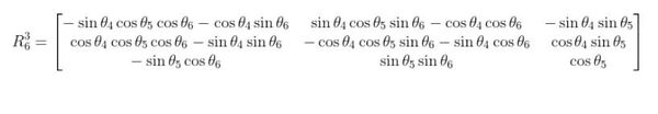
To calculate the rotation of frame 6 relative to frame 3, we need to go back to the kinematic diagram we drew earlier.
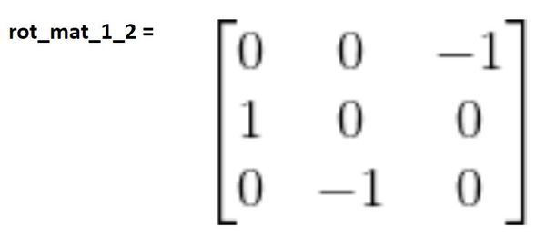
Using either the rotation matrix method or Denavit-Hartenberg, here is the rotation matrix you get when you consider just the frames from 3 to 6.
Determine rot_mat_0_6
Now, let’s determine the rotation matrix of frame 6 relative to frame 0, the global coordinate frame.

In this part, we need to determine what we want the orientation of the end effector to be so that we can define the rotation matrix of frame 6 relative to frame 0. We can choose any rotation matrix as long as it is a valid rotation matrix (I’ll explain what “valid” means below).
Imagine you want the end effector to point upwards towards the sky. In this case, z6 will point in the same direction as z0. Accordingly, if you can imagine z6 pointing straight upwards, x6 would be oriented in the opposite direction as x0, and y6 would be oriented in the opposite direction as y0. Our rotation matrix is thus:
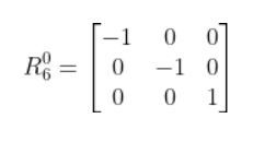
The rotation matrix above is valid. The reason it is valid is because the length (also known as “norm” or “magnitude”) of each row and each column is 1. The length of a column or row is the square root of the sum of the squared elements.
For example, looking at column 1, we have:

Write Python Code
Open up your favorite Python IDE or wherever you like to write Python code.
Create up a new Python script. Call it inverse_kinematics_6dof_v1.py.
We want to set a desired position and orientation (relative to the base frame) for the end effector of the robotic arm and then have the program calculate the servo angles necessary to move the end effector to that position and orientation.
Write the following code. These expressions and matrices below (that we derived earlier) will be useful to you as you go through the code. Don’t be intimidated at how long the code is. Just copy and paste it into your favorite Python IDE or text editor, and read through it one line at a time.
#######################################################################################
# Progam: Inverse Kinematics for a 6DOF Robotic Arm Using an Analytical Approach
# Description: Given a desired end position (x, y, z) of the end effector of a robot,
# and a desired orientation of the end effector (relative to the base frame),
# calculate the joint angles (i.e. angles for the servo motors).
# Author: Addison Sears-Collins
# Website: https://automaticaddison.com
# Date: October 19, 2020
# Reference: Sodemann, Dr. Angela 2020, RoboGrok, accessed 14 October 2020, <http://robogrok.com/>
#######################################################################################
import numpy as np # Scientific computing library
# Define the desired position of the end effector
# This is the target (goal) location.
x = 4.0
y = 2.0
# Calculate the angle of the second joint
theta_2 = np.arctan2(y,x)
print(f'Theta 2 = {theta_2} radians\n')
# Define the desired orientation of the end effector relative to the base frame
# (i.e. global frame)
# This is the target orientation.
# The 3x3 rotation matrix of frame 6 relative to frame 0
rot_mat_0_6 = np.array([[-1.0, 0.0, 0.0],
[0.0, -1.0, 0.0],
[0.0, 0.0, 1.0]])
# The 3x3 rotation matrix of frame 3 relative to frame 0
rot_mat_0_3 = np.array([[-np.sin(theta_2), 0.0, np.cos(theta_2)],
[np.cos(theta_2), 0.0, np.sin(theta_2)],
[0.0, 1.0, 0.0]])
# Calculate the inverse rotation matrix
inv_rot_mat_0_3 = np.linalg.inv(rot_mat_0_3)
# Calculate the 3x3 rotation matrix of frame 6 relative to frame 3
rot_mat_3_6 = inv_rot_mat_0_3 @ rot_mat_0_6
print(f'rot_mat_3_6 = {rot_mat_3_6}')
# We know the equation for rot_mat_3_6 from our pencil and paper
# analysis. The simplest term in that matrix is in the third column,
# third row. The value there in variable terms is cos(theta_5).
# From the printing above, we know the value there. Therefore,
# cos(theta_5) = value in the third row, third column of rot_mat_3_6, which means...
# theta_5 = arccosine(value in the third row, third column of rot_mat_3_6)
theta_5 = np.arccos(rot_mat_3_6[2, 2])
print(f'\nTheta 5 = {theta_5} radians')
# Calculate the value for theta_6
# We'll use the expression in the third row, first column of rot_mat_3_6.
# -sin(theta_5)cos(theta_6) = rot_mat_3_6[2,0]
# Solving for theta_6...
# rot_mat_3_6[2,0]/-sin(theta_5) = cos(theta_6)
# arccosine(rot_mat_3_6[2,0]/-sin(theta_5)) = theta_6
theta_6 = np.arccos(rot_mat_3_6[2, 0] / -np.sin(theta_5))
print(f'\nTheta 6 = {theta_6} radians')
# Calculate the value for theta_4 using one of the other
# cells in rot_mat_3_6. We'll use the second row, third column.
# cos(theta_4)sin(theta_5) = rot_mat_3_6[1,2]
# cos(theta_4) = rot_mat_3_6[1,2] / sin(theta_5)
# theta_4 = arccosine(rot_mat_3_6[1,2] / sin(theta_5))
theta_4 = np.arccos(rot_mat_3_6[1,2] / np.sin(theta_5))
print(f'\nTheta 4 = {theta_4} radians')
# Check that the angles we calculated result in a valid rotation matrix
r11 = -np.sin(theta_4) * np.cos(theta_5) * np.cos(theta_6) - np.cos(theta_4) * np.sin(theta_6)
r12 = np.sin(theta_4) * np.cos(theta_5) * np.sin(theta_6) - np.cos(theta_4) * np.cos(theta_6)
r13 = -np.sin(theta_4) * np.sin(theta_5)
r21 = np.cos(theta_4) * np.cos(theta_5) * np.cos(theta_6) - np.sin(theta_4) * np.sin(theta_6)
r22 = -np.cos(theta_4) * np.cos(theta_5) * np.sin(theta_6) - np.sin(theta_4) * np.cos(theta_6)
r23 = np.cos(theta_4) * np.sin(theta_5)
r31 = -np.sin(theta_5) * np.cos(theta_6)
r32 = np.sin(theta_5) * np.sin(theta_6)
r33 = np.cos(theta_5)
check_rot_mat_3_6 = np.array([[r11, r12, r13],
[r21, r22, r23],
[r31, r32, r33]])
# Original matrix
print(f'\nrot_mat_3_6 = {rot_mat_3_6}')
# Check Matrix
print(f'\ncheck_rot_mat_3_6 = {check_rot_mat_3_6}\n')
# Return if Original Matrix == Check Matrix
rot_minus_check_3_6 = rot_mat_3_6.round() - check_rot_mat_3_6.round()
zero_matrix = np.array([[0, 0, 0],
[0, 0, 0],
[0, 0, 0]])
matrices_are_equal = np.array_equal(rot_minus_check_3_6, zero_matrix)
# Determine if the solution is valid or not
# If the solution is valid, that means the end effector of the robotic
# arm can reach that target location.
if (matrices_are_equal):
valid_matrix = "Yes"
else:
valid_matrix = "No"
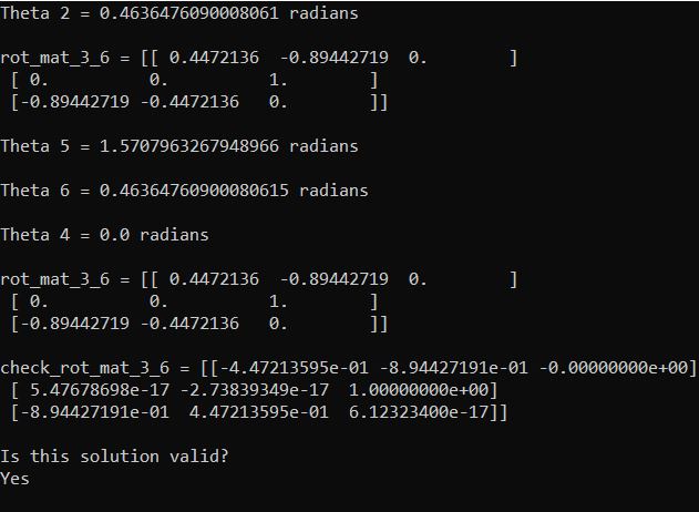
print(f'Is this solution valid?\n{valid_matrix}\n')
Here is the output:
References
Sodemann, Dr. Angela 2020, RoboGrok, accessed 14 October 2020, <http://robogrok.com/>
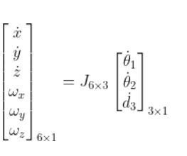
Inverse Kinematics Using the Pseudoinverse Jacobian Method (Numerical Approach)
Let’s take a look at a numerical approach to inverse kinematics. There are a number of approaches, but in this section will explore one that is quite popular in industry and academia: the Pseudoinverse Jacobian Method.
This method is called “numerical” because it involves iteration to calculate the joint angles from the desired end effector position.
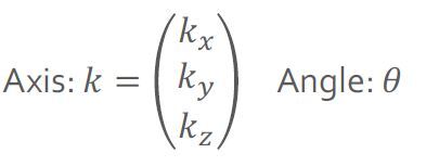
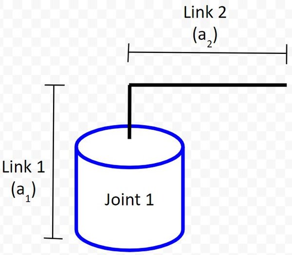
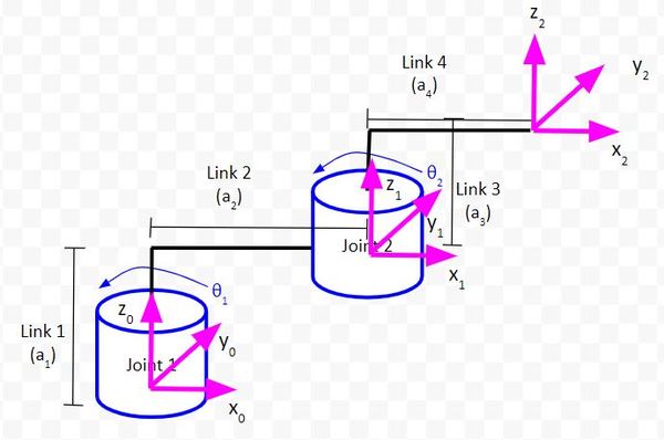
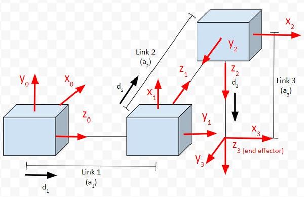
We’ll take a look at a SCARA-like robotic arm below that has 2 degrees of freedom (two joints/motors and 4 links).
To extend this example to a 6DOF robotic arm, just add 4 more joints and the appropriate number of links. Make sure before you do this step, that you’ve drawn the kinematic diagram. On this page, I have several examples of kinematic diagrams for 6DOF robotic arms.
Full Code in Python
Here is the full code. I named the program inv_kinematics_using_pseudo_jacobian.py. I’ll explain each piece step-by-step below.
#######################################################################################
# Progam: Inverse Kinematics for a Robotic Arm Using the Pseudoinverse of the Jacobian
# Description: Given a desired end position (x, y, z) of the end effector of a robot,
# calculate the joint angles (i.e. angles for the servo motors).
# Author: Addison Sears-Collins
# Website: https://automaticaddison.com
# Date: October 15, 2020
#######################################################################################
import numpy as np # Scientific computing library
def axis_angle_rot_matrix(k,q):
"""
Creates a 3x3 rotation matrix in 3D space from an axis and an angle.
Input
:param k: A 3 element array containing the unit axis to rotate around (kx,ky,kz)
:param q: The angle (in radians) to rotate by
Output
:return: A 3x3 element matix containing the rotation matrix
"""
#15 pts
c_theta = np.cos(q)
s_theta = np.sin(q)
v_theta = 1 - np.cos(q)
kx = k[0]
ky = k[1]
kz = k[2]
# First row of the rotation matrix
r00 = kx * kx * v_theta + c_theta
r01 = kx * ky * v_theta - kz * s_theta
r02 = kx * kz * v_theta + ky * s_theta
# Second row of the rotation matrix
r10 = kx * ky * v_theta + kz * s_theta
r11 = ky * ky * v_theta + c_theta
r12 = ky * kz * v_theta - kx * s_theta
# Third row of the rotation matrix
r20 = kx * kz * v_theta - ky * s_theta
r21 = ky * kz * v_theta + kx * s_theta
r22 = kz * kz * v_theta + c_theta
# 3x3 rotation matrix
rot_matrix = np.array([[r00, r01, r02],
[r10, r11, r12],
[r20, r21, r22]])
return rot_matrix
def hr_matrix(k,t,q):
'''
Create the Homogenous Representation matrix that transforms a point from Frame B to Frame A.
Using the axis-angle representation
Input
:param k: A 3 element array containing the unit axis to rotate around (kx,ky,kz)
:param t: The translation from the current frame (e.g. Frame A) to the next frame (e.g. Frame B)
:param q: The rotation angle (i.e. joint angle)
Output
:return: A 4x4 Homogenous representation matrix
'''
# Calculate the rotation matrix (angle-axis representation)
rot_matrix_A_B = axis_angle_rot_matrix(k,q)
# Store the translation vector t
translation_vec_A_B = t
# Convert to a 2D matrix
t0 = translation_vec_A_B[0]
t1 = translation_vec_A_B[1]
t2 = translation_vec_A_B[2]
translation_vec_A_B = np.array([[t0],
[t1],
[t2]])
# Create the homogeneous transformation matrix
homgen_mat = np.concatenate((rot_matrix_A_B, translation_vec_A_B), axis=1) # side by side
# Row vector for bottom of homogeneous transformation matrix
extra_row_homgen = np.array([[0, 0, 0, 1]])
# Add extra row to homogeneous transformation matrix
homgen_mat = np.concatenate((homgen_mat, extra_row_homgen), axis=0) # one above the other
return homgen_mat
class RoboticArm:
def __init__(self,k_arm,t_arm):
'''
Creates a robotic arm class for computing position and velocity.
Input
:param k_arm: A 2D array that lists the different axes of rotation (rows) for each joint.
:param t_arm: A 2D array that lists the translations from the previous joint to the current joint
The first translation is from the global (base) frame to joint 1 (which is often equal to the global frame)
The second translation is from joint 1 to joint 2, etc.
'''
self.k = np.array(k_arm)
self.t = np.array(t_arm)
assert k_arm.shape == t_arm.shape, 'Warning! Improper definition of rotation axes and translations'
self.N_joints = k_arm.shape[0]
def position(self,Q,index=-1,p_i=[0,0,0]):
'''
Compute the position in the global (base) frame of a point given in a joint frame
(default values will assume the input position vector is in the frame of the last joint)
Input
:param p_i: A 3 element vector containing a position in the frame of the index joint
:param index: The index of the joint frame being converted from (first joint is 0, the last joint is N_joints - 1)
Output
:return: A 3 element vector containing the new position with respect to the global (base) frame
'''
# The position of this joint described by the index
p_i_x = p_i[0]
p_i_y = p_i[1]
p_i_z = p_i[2]
this_joint_position = np.array([[p_i_x],
[p_i_y],
[p_i_z],
[1]])
# End effector joint
if (index == -1):
index = self.N_joints - 1
# Store the original index of this joint
orig_joint_index = index
# Store the result of matrix multiplication
running_multiplication = None
# Start from the index of this joint and work backwards to index 0
while (index >= 0):
# If we are at the original joint index
if (index == orig_joint_index):
running_multiplication = hr_matrix(self.k[index],self.t[index],Q[index]) @ this_joint_position
# If we are not at the original joint index
else:
running_multiplication = hr_matrix(self.k[index],self.t[index],Q[index]) @ running_multiplication
index = index - 1
# extract the points
px = running_multiplication[0][0]
py = running_multiplication[1][0]
pz = running_multiplication[2][0]
position_global_frame = np.array([px, py, pz])
return position_global_frame
def pseudo_inverse(self,theta_start,p_eff_N,goal_position,max_steps=np.inf):
'''
Performs the inverse kinematics using the pseudoinverse of the Jacobian
:param theta_start: An N element array containing the current joint angles in radians (e.g. np.array([np.pi/8,np.pi/4,np.pi/6]))
:param p_eff_N: A 3 element vector containing translation from the last joint to the end effector in the last joints frame of reference
:param goal_position: A 3 element vector containing the desired end position for the end effector in the global (base) frame
:param max_steps: (Optional) Maximum number of iterations to compute
Output
:return: An N element vector containing the joint angles that result in the end effector reaching xend (i.e. the goal)
'''
v_step_size = 0.05
theta_max_step = 0.2
Q_j = theta_start # Array containing the starting joint angles
p_end = np.array([goal_position[0], goal_position[1], goal_position[2]]) # desired x, y, z coordinate of the end effector in the base frame
p_j = self.position(Q_j,p_i=p_eff_N) # x, y, z coordinate of the position of the end effector in the global reference frame
delta_p = p_end - p_j # delta_x, delta_y, delta_z between start position and desired final position of end effector
j = 0 # Initialize the counter variable
# While the magnitude of the delta_p vector is greater than 0.01
# and we are less than the max number of steps
while np.linalg.norm(delta_p) > 0.01 and j<max_steps:
print(f'j{j}: Q[{Q_j}] , P[{p_j}]') # Print the current joint angles and position of the end effector in the global frame
# Reduce the delta_p 3-element delta_p vector by some scaling factor
# delta_p represents the distance between where the end effector is now and our goal position.
v_p = delta_p * v_step_size / np.linalg.norm(delta_p)
# Get the jacobian matrix given the current joint angles
J_j = self.jacobian(Q_j,p_eff_N)
# Calculate the pseudo-inverse of the Jacobian matrix
J_invj = np.linalg.pinv(J_j)
# Multiply the two matrices together
v_Q = np.matmul(J_invj,v_p)
# Move the joints to new angles
# We use the np.clip method here so that the joint doesn't move too much. We
# just want the joints to move a tiny amount at each time step because
# the full motion of the end effector is nonlinear, and we're approximating the
# big nonlinear motion of the end effector as a bunch of tiny linear motions.
Q_j = Q_j + np.clip(v_Q,-1*theta_max_step,theta_max_step)#[:self.N_joints]
# Get the current position of the end-effector in the global frame
p_j = self.position(Q_j,p_i=p_eff_N)
# Increment the time step
j = j + 1
# Determine the difference between the new position and the desired end position
delta_p = p_end - p_j
# Return the final angles for each joint
return Q_j
def jacobian(self,Q,p_eff_N=[0,0,0]):
'''
Computes the Jacobian (just the position, not the orientation)
:param Q: An N element array containing the current joint angles in radians
:param p_eff_N: A 3 element vector containing translation from the last joint to the end effector in the last joints frame of reference
Output
:return: A 3xN 2D matrix containing the Jacobian matrix
'''
# Position of the end effector in global frame
p_eff = self.position(Q,-1,p_eff_N)
first_iter = True
jacobian_matrix = None
for i in range(0, self.N_joints):
if (first_iter == True):
# Difference in the position of the end effector in the global frame
# and this joint in the global frame
p_eff_minus_this_p = p_eff - self.position(Q,index=i)
# Axes
kx = self.k[i][0]
ky = self.k[i][1]
kz = self.k[i][2]
k = np.array([kx, ky, kz])
px = p_eff_minus_this_p[0]
py = p_eff_minus_this_p[1]
pz = p_eff_minus_this_p[2]
p_eff_minus_this_p = np.array([px, py, pz])
this_jacobian = np.cross(k, p_eff_minus_this_p)
# Convert to a 2D matrix
j0 = this_jacobian[0]
j1 = this_jacobian[1]
j2 = this_jacobian[2]
this_jacobian = np.array([[j0],
[j1],
[j2]])
jacobian_matrix = this_jacobian
first_iter = False
else:
p_eff_minus_this_p = p_eff - self.position(Q,index=i)
# Axes
kx = self.k[i][0]
ky = self.k[i][1]
kz = self.k[i][2]
k = np.array([kx, ky, kz])
# Difference between this joint's position and end effector's position
px = p_eff_minus_this_p[0]
py = p_eff_minus_this_p[1]
pz = p_eff_minus_this_p[2]
p_eff_minus_this_p = np.array([px, py, pz])
this_jacobian = np.cross(k, p_eff_minus_this_p)
# Convert to a 2D matrix
j0 = this_jacobian[0]
j1 = this_jacobian[1]
j2 = this_jacobian[2]
this_jacobian = np.array([[j0],
[j1],
[j2]])
jacobian_matrix = np.concatenate((jacobian_matrix, this_jacobian), axis=1) # side by side
return jacobian_matrix
def main():
'''Given a two degree of freedom robotic arm and a desired end position of the end effector,
calculate the two joint angles (i.e. servo angles).
'''
# A 2D array that lists the different axes of rotation (rows) for each joint
# Here I assume our robotic arm has two joints, but you can add more if you like.
# k = kx, ky, kz
k = np.array([[0,0,1],[0,0,1]])
# A 2D array that lists the translations from the previous joint to the current joint
# The first translation is from the base frame to joint 1 (which is equal to the base frame)
# The second translation is from joint 1 to joint 2
# t = tx, ty, tz
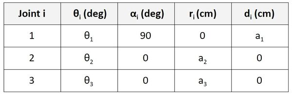
# These values are measured with a ruler based on the kinematic diagram
# This tutorial teaches you how to draw kinematic diagrams:
# https://automaticaddison.com/how-to-assign-denavit-hartenberg-frames-to-robotic-arms/
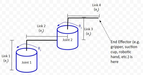
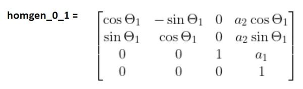
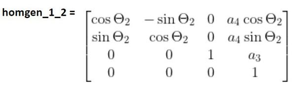
a1 = 4.7
a2 = 5.9
a3 = 5.4
a4 = 6.0
t = np.array([[0,0,0],[a2,0,a1]])
# Position of end effector in joint 2 (i.e. the last joint) frame
p_eff_2 = [a4,0,a3]
# Create an object of the RoboticArm class
k_c = RoboticArm(k,t)
# Starting joint angles in radians (joint 1, joint 2)
q_0 = np.array([0,0])
# desired end position for the end effector with respect to the base frame of the robotic arm
endeffector_goal_position = np.array([4.0,10.0,a1 + a4])
# Display the starting position of each joint in the global frame
for i in np.arange(0,k_c.N_joints):
print(f'joint {i} position = {k_c.position(q_0,index=i)}')
print(f'end_effector = {k_c.position(q_0,index=-1,p_i=p_eff_2)}')
print(f'goal = {endeffector_goal_position}')
# Return joint angles that result in the end effector reaching endeffector_goal_position
final_q = k_c.pseudo_inverse(q_0, p_eff_N=p_eff_2, goal_position=endeffector_goal_position, max_steps=500)
# Final Joint Angles in degrees
print('\n\nFinal Joint Angles in Degrees')
print(f'Joint 1: {np.degrees(final_q[0])} , Joint 2: {np.degrees(final_q[1])}')
if __name__ == '__main__':
main()
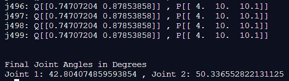
Here is the output:
axis_angle_rot_matrix(k,q)
There are multiple ways to describe rotation in a robotic system. In previous tutorial, I have covered some of those methods:
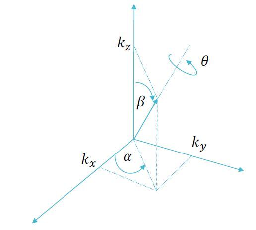
Another way to describe rotation in a robotic system is to use the Axis-Angle representation. With this representation, any orientation of a robotic system in three dimensions is equivalent to a rotation about a fixed axis k through angle θ.
For example, suppose you have a base frame of a robotic arm. This frame is Frame 0 (Joint 1).
The next frame (i.e. the next joint or servo motor) would be Frame 1 (Joint 2). Frame 1 of the robotic arm would be rotated around axis k by angle θ1.
In most of my robotics work, I’ve assumed that rotation at any joint is around the z axis. So, in this code, I’ve assumed that axis k is the following vector.
k = (kx, ky, kz) = (0, 0, 1)
With the rotation around that axis being θ (e.g. θ1, θ2, θ3, etc.).
Given axis-angle representation, the equivalent 3×3 rotation matrix Rk(θ) is as follows:
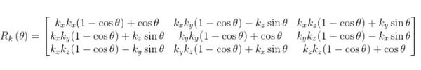
This equation above is what you see implemented in the code.
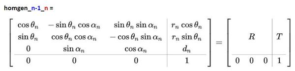
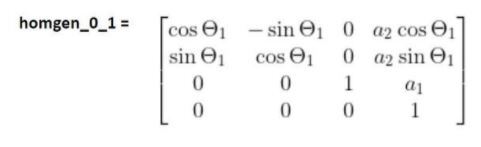
hr_matrix(k,t,q)
This code creates the homogeneous representation (also called “transformation”) matrix. A homogeneous rotation matrix combines the rotation and translation (i.e. displacement) of one coordinate frame relative to another coordinate frame into a single 4 row x 4 column matrix.
class RoboticArm
This class represents the robotic arm that we want to control.
__init__(self,k_arm,t_arm)
This piece of code is the constructor for the robotic arm class. This constructor initializes the data fields of the robotic arm of interest. These data fields include the number of joints, the rotation axes for each joint, and the measured lengths (i.e. translations) between each joint.
position(self,Q,index=-1,p_i=[0,0,0])
This piece of code uses hr_matrix(k,t,q) to calculate the position in the global (base) frame of a point given in a joint frame.
pseudo_inverse(self,theta_start,p_eff_N,goal_position,max_steps=np.inf)
This piece of code performs inverse kinematics using the pseudoinverse of the Jacobian. What does that mean? Let me explain now how this process works.
You start off with the joints of the robotic arm at arbitrary angles (by convention I typically set them to 0 degrees).
The end effector of the robotic arm is located at some arbitrary position in 3D space.
You then iterate. At each step of the iteration, you
1. Calculate the distance between the current end effector position and the desired goal end effector position. This value (which is a vector…a list of numbers) is often called “delta p”.
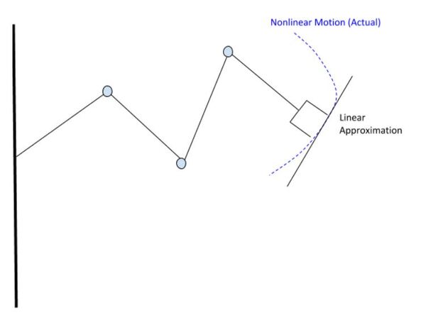
2. Reduce the delta p vector by some scaling factor so that it is really small. We only want the end effector to move by a small amount at each time step because, for small motions, we can approximate the displacement of the end effector as linear. Doing this makes the math easier, enabling us to use the Jacobian matrix. The Jacobian matrix is, at its core, is a matrix of partial derivatives.
Remember, forward kinematics (i.e. the motion of revolute joints like servo motors) is nonlinear and would typically involve sines and cosines like we saw in the Analytical IK method), but in this case, we make linear approximations to that nonlinear motion.
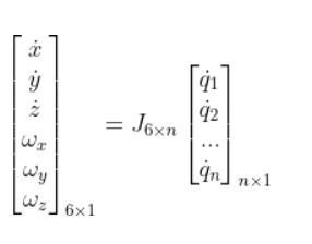
3. Calculate the Jacobian matrix J.
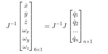
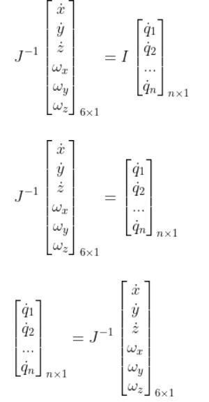
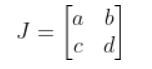
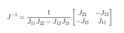
4, Calculate the pseudoinverse of the Jacobian matrix. The pseudoinverse of the Jacobian matrix is calculated because the regular inverse (i.e. J-1 which we looked at in a previous tutorial) fails if a matrix is not square (i.e. a square matrix is a matrix with the same number of columns and rows). The pseudoinverse can invert a non-square matrix.
5. Multiply the pseudoinverse of the Jacobian matrix and the scaled delta p vector together to calculate the desired tiny change in the joint values.
6. Update each joint angle by the amount of that tiny change.
7. The resulting motion from updating the joint values should bring the end effector just a little bit closer to your desired goal position.
Keep repeating the steps above again and again until the end effector has reached the desired goal position (or rather “close enough”).
In a nutshell, at each iteration, we have the end effector take tiny steps towards the goal. We only stop when the end effector reaches the goal position.
I like to set the maximum number of iterations around 500, but you’ll often get the end effector to reach the desired goal position long before that many iterations.
Once the end effector is close enough, return the final joint angles. For a real robotic arm, these are the angles that each servo motor would need to be for the end effector of the arm to be at the goal position.
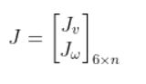
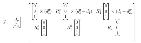
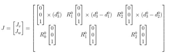
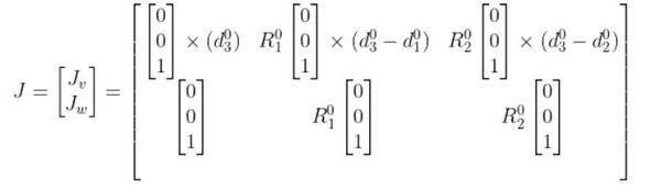
jacobian(self,Q,p_eff_N=[0,0,0])
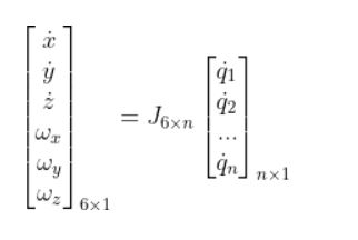
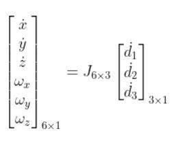
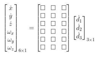
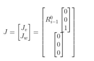
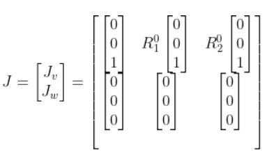
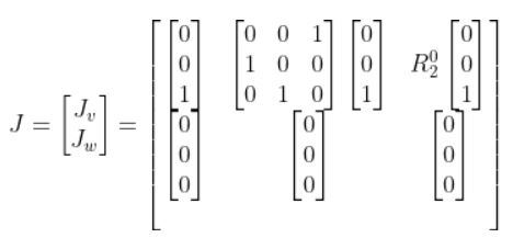
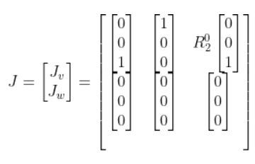
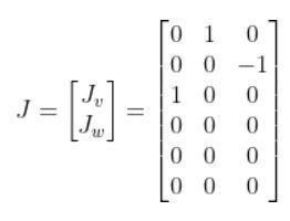
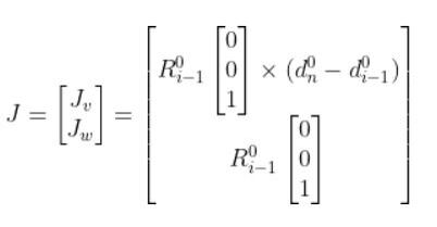
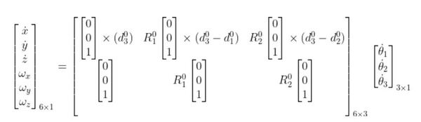
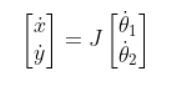
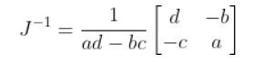
In this piece of code, we calculate the Jacobian matrix (position part on the top half…not the orientation part on the bottom half).
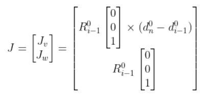
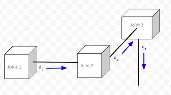
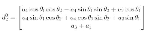
d0n is the displacement from the origin of the global coordinate frame to the origin of the end of the end effector.
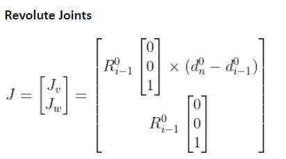
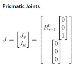
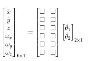
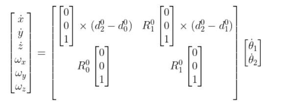
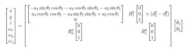
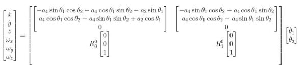
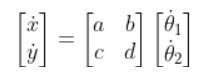
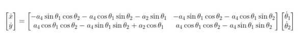
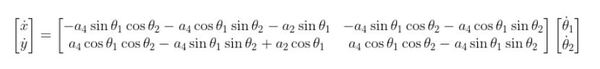
For a revolute joint (like a servo motor), the change in the linear velocity of the end effector is the cross product of the axis of revolution k (which is made up of 3 elements, kx, ky, and kz) and a 3-element position vector from the joint to the end effector.
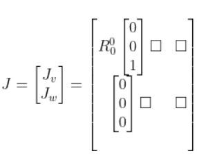
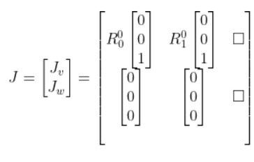
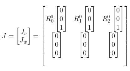
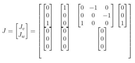
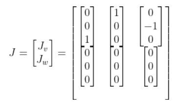
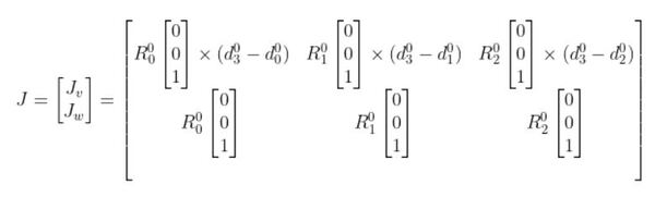
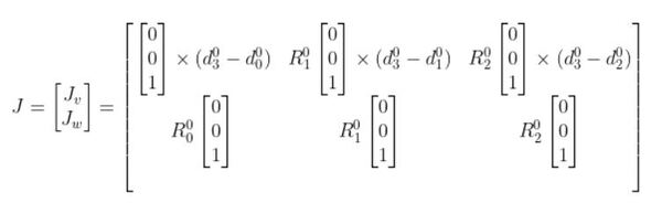
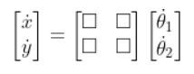
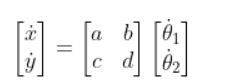
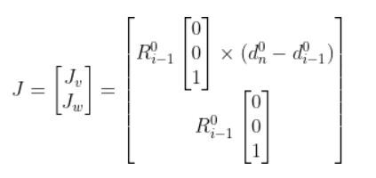
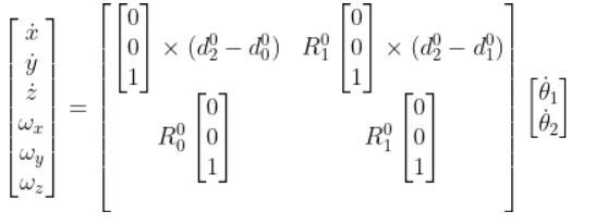
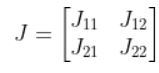
For example, given a robotic arm with two joints (i.e. two servo motors), the Jacobian is calculated as follows:
Jv = [Jv1, Jv2]
Where:
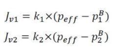
- Jv1 is the first column of the Jacobian matrix.
- Jv2 is the second column of the Jacobian matrix.
- k1 is the 3-element axis for the first joint (e.g. (0, 0, 1)).
- k2 is the 3-element axis for the second joint (e.g. (0, 0, 1)).
- peff is a 3-element vector that represents the position of the end effector in the base frame of the robotic arm.
- pB1 is the position of joint 1 relative to the base frame.
- pB2 is the position of joint 2 relative to the base frame.
main()
Given a two degree of freedom robotic arm and a desired end position of the end effector, we calculate the two joint angles (i.e. servo angles).
If you see this line of code, you’ll see that I want the robotic arm to go to x = 4.0, y = 10.0.
endeffector_goal_position = np.array([4.0,10.0,a1 + a4])
In fact, these coordinates are the same goal coordinates I set in this inverse kinematics project, where I did an analytical approach to inverse kinematics on a real robotic arm.
In that post, I set the goal destination to x = 4.0 and y = 10.0. If you uncomment the Arduino code on that tutorial and run it, you’ll see that the Serial Monitor outputs the final joint angles (that get the end effector of the robotic arm to the goal destination) as:
θ1 = 42.8
θ2 = 50.3
This is pretty much equal to what we get with the Pseudoinverse Jacobian approach from our Python code earlier in this section.
Conclusion
What I’ve shown in this tutorial are two popular methods for calculating the inverse kinematics of a robotic arm. There are other methods out there like Cyclic Coordinate Descent, the Damped Least Squares method, and the Jacobian Transpose method. What method you choose for your project depends on your personal preference and what you’re trying to achieve.
That’s it! Keep building!


