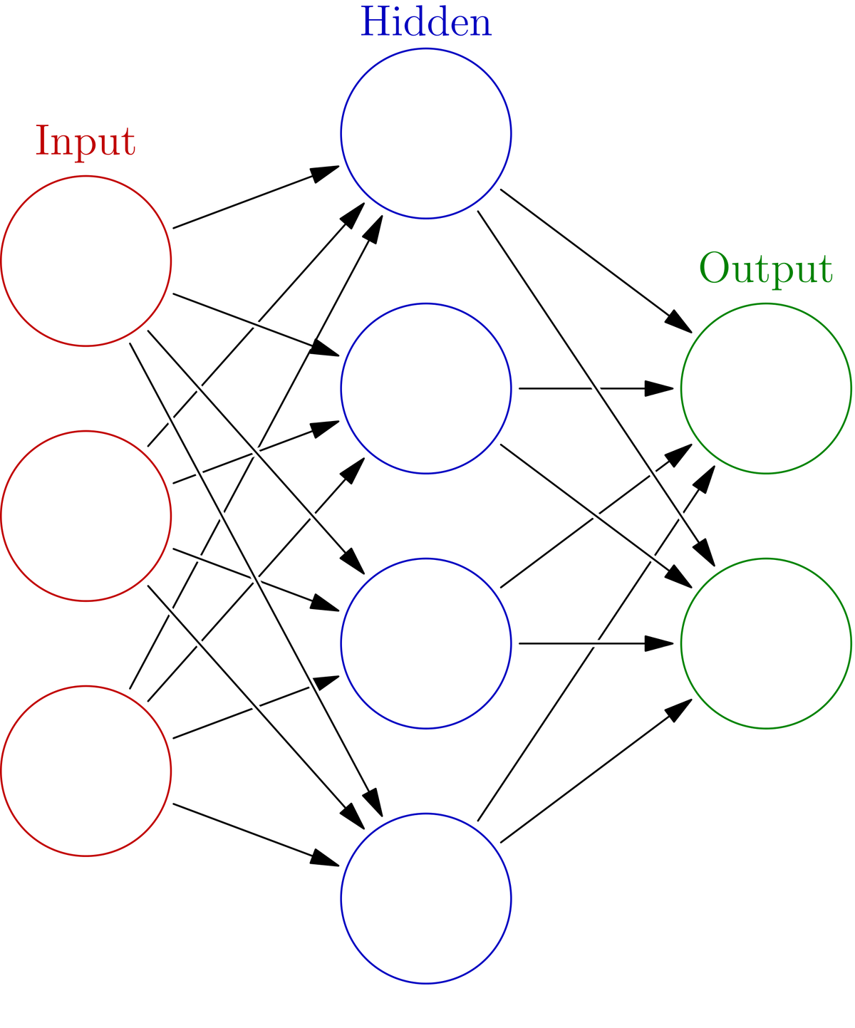
In this tutorial, we will use Tensorflow 2.0 with Keras to build a deep neural network that will enable us to predict a vehicle’s fuel economy (in miles per gallon) from eight different attributes:
- Cylinders
- Displacement
- Horsepower
- Weight
- Acceleration
- Model year
- Origin
- Car name
We will use the Auto MPG Data Set at the UCI Machine Learning Repository.
Prerequisites
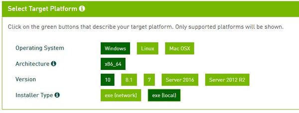
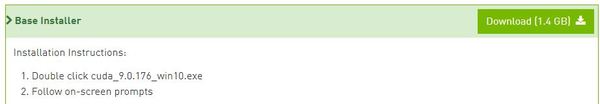
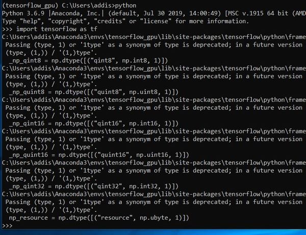
- You have TensorFlow 2 Installed.
- Windows 10 Users, see this post.
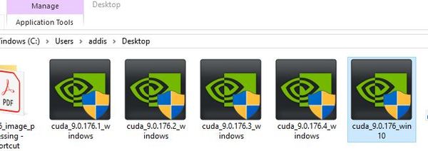
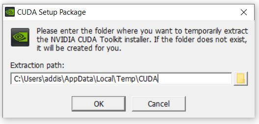
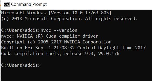
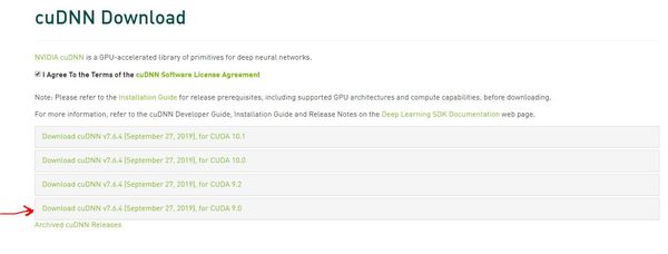
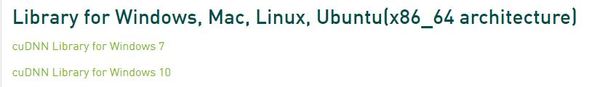
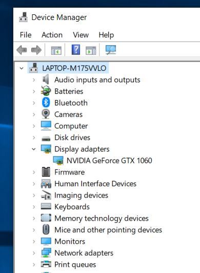
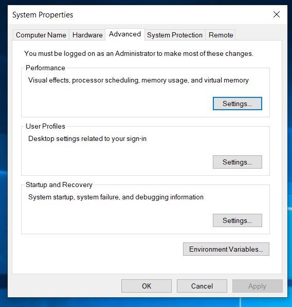
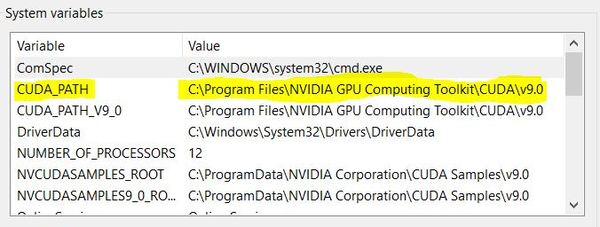
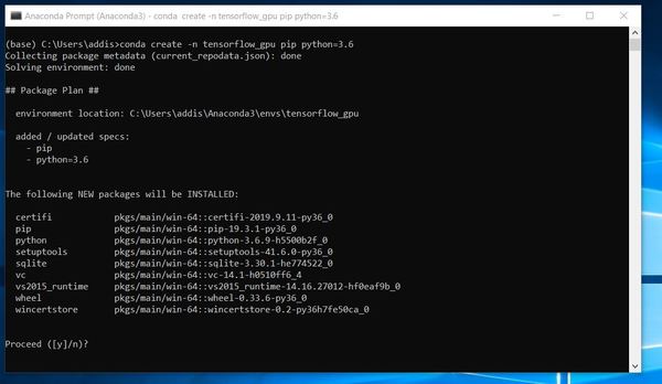
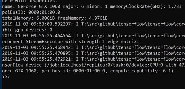
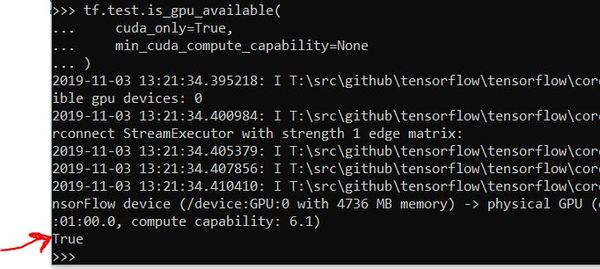
- If you want to use GPU support for your TensorFlow installation, you will need to follow these steps. If you have trouble following those steps, you can follow these steps (note that the steps change quite frequently, but the overall process remains relatively the same).
Directions
Open up a new Python program (in your favorite text editor or Python IDE) and write the following code. I’m going to name the program vehicle_fuel_economy.py. I’ll explain the code later in this tutorial.
# Project: Predict Vehicle Fuel Economy Using a Deep Neural Network
# Author: Addison Sears-Collins
# Date created: November 3, 2020
import pandas as pd # Used for data analysis
import pathlib # An object-oriented interface to the filesystem
import matplotlib.pyplot as plt # Handles the creation of plots
import seaborn as sns # Data visualization library
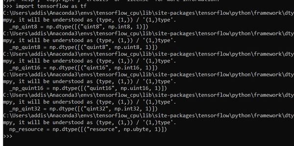
import tensorflow as tf # Machine learning library
from tensorflow import keras # Library for neural networks
from tensorflow.keras import layers # Handles the layers of the neural network
def main():
# Set the data path for the Auto-Mpg data set from the UCI Machine Learning Repository
datasetPath = keras.utils.get_file("auto-mpg.data", "https://archive.ics.uci.edu/ml/machine-learning-databases/auto-mpg/auto-mpg.data")
# Set the column names for the data set
columnNames = ['MPG', 'Cylinders','Displacement','Horsepower','Weight',
'Acceleration','Model Year','Origin']
# Import the data set
originalData = pd.read_csv(datasetPath, names=columnNames, na_values = "?",
comment='\t', sep=" ", skipinitialspace=True)
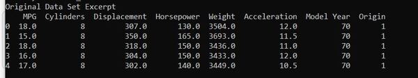
# Check the data set
# print("Original Data Set Excerpt")
# print(originalData.head())
# print()
# Generate a copy of the data set
data = originalData.copy()
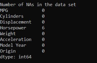
# Count how many NAs each data attribute has
# print("Number of NAs in the data set")
# print(data.isna().sum())
# print()
# Now, let's remove the NAs from the data set
data = data.dropna()
# Perform one-hot encoding on the Origin attribute
# since it is a categorical variable
origin = data.pop('Origin') # Return item and drop from frame
data['USA'] = (origin == 1) * 1.0
data['Europe'] = (origin == 2) * 1.0
data['Japan'] = (origin == 3) * 1.0
# Generate a training data set (80% of the data) and a testing set (20% of the data)
trainingData = data.sample(frac = 0.8, random_state = 0)
# Generate a testing data set
testingData = data.drop(trainingData.index)
# Separate the attributes from the label in both the testing
# and training data. The label is the thing we are trying
# to predit (i.e. miles per gallon 'MPG')
trainingLabelData = trainingData.pop('MPG')
testingLabelData = testingData.pop('MPG')
# Normalize the data
normalizedTrainingData = normalize(trainingData)
normalizedTestingData = normalize(testingData)
#print(normalizedTrainingData.head())
# Generate the neural network
neuralNet = generateNeuralNetwork(trainingData)
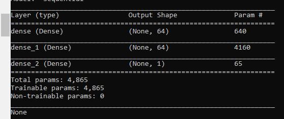
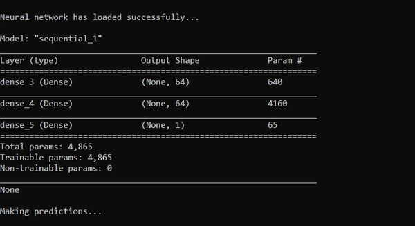
# See a summary of the neural network
# The first layer has 640 parameters
#(9 input values * 64 neurons) + 64 bias values
# The second layer has 4160 parameters
#(64 input values * 64 neurons) + 64 bias values
# The output layer has 65 parameters
#(64 input values * 1 neuron) + 1 bias value
#print(neuralNet.summary())
EPOCHS = 1000
# Train the model for a fixed number of epochs
# history.history attribute is returned from the fit() function.
# history.history is a record of training loss values and
# metrics values at successive epochs, as well as validation
# loss values and validation metrics values.
history = neuralNet.fit(
x = normalizedTrainingData,
y = trainingLabelData,
epochs = EPOCHS,
validation_split = 0.2,
verbose = 0,
callbacks = [PrintDot()]
)
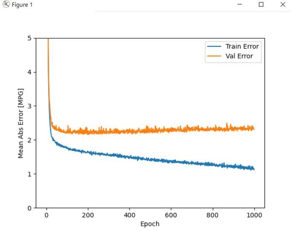
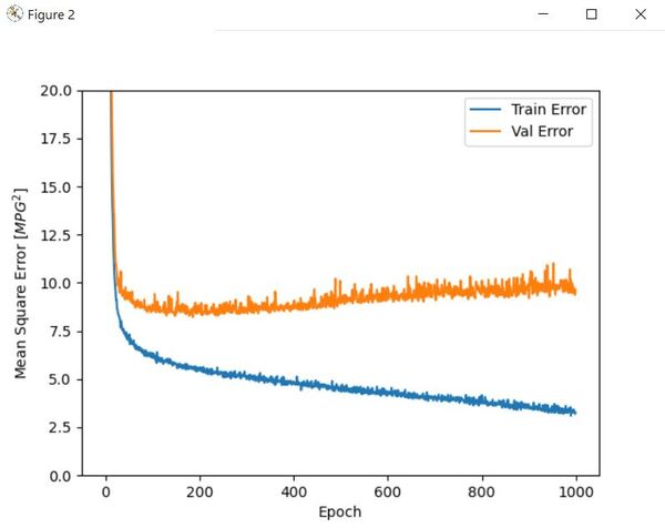
# Plot the neural network metrics (Training error and validation error)
# Training error is the error when the trained neural network is
# run on the training data.
# Validation error is used to minimize overfitting. It indicates how
# well the data fits on data it hasn't been trained on.
#plotNeuralNetMetrics(history)
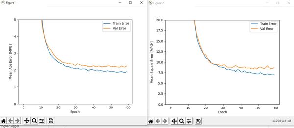
# Generate another neural network so that we can use early stopping
neuralNet2 = generateNeuralNetwork(trainingData)
# We want to stop training the model when the
# validation error stops improving.
# monitor indicates the quantity we want to monitor.
# patience indicates the number of epochs with no improvement after which
# training will terminate.
earlyStopping = keras.callbacks.EarlyStopping(monitor = 'val_loss', patience = 10)
history2 = neuralNet2.fit(
x = normalizedTrainingData,
y = trainingLabelData,
epochs = EPOCHS,
validation_split = 0.2,
verbose = 0,
callbacks = [earlyStopping, PrintDot()]
)
# Plot metrics
#plotNeuralNetMetrics(history2)
# Return the loss value and metrics values for the model in test mode
# The mean absolute error for the predictions should
# stabilize around 2 miles per gallon
loss, meanAbsoluteError, meanSquaredError = neuralNet2.evaluate(
x = normalizedTestingData,
y = testingLabelData,
verbose = 0
)
#print(f'\nMean Absolute Error on Test Data Set = {meanAbsoluteError} miles per gallon')
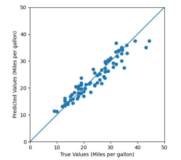
# Make fuel economy predictions by deploying the trained neural network on the
# test data set (data that is brand new for the trained neural network).
testingDataPredictions = neuralNet2.predict(normalizedTestingData).flatten()
# Plot the predicted MPG vs. the true MPG
# testingLabelData are the true MPG values
# testingDataPredictions are the predicted MPG values
#plotTestingDataPredictions(testingLabelData, testingDataPredictions)
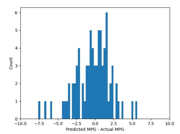
# Plot the prediction error distribution
#plotPredictionError(testingLabelData, testingDataPredictions)
# Save the neural network in Hierarchical Data Format version 5 (HDF5) format
neuralNet2.save('fuel_economy_prediction_nnet.h5')
# Import the saved model
neuralNet3 = keras.models.load_model('fuel_economy_prediction_nnet.h5')
print("\n\nNeural network has loaded successfully...\n")
# Show neural network parameters
print(neuralNet3.summary())
# Make a prediction using the saved model we just imported
print("\nMaking predictions...")
testingDataPredictionsNN3 = neuralNet3.predict(normalizedTestingData).flatten()
# Show Predicted MPG vs. Actual MPG
plotTestingDataPredictions(testingLabelData, testingDataPredictionsNN3)
# Generate the neural network
def generateNeuralNetwork(trainingData):
# A Sequential model is a stack of layers where each layer is
# single-input, single-output
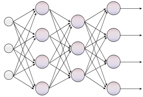
# This network below has 3 layers.
neuralNet = keras.Sequential([
# Each neuron in a layer recieves input from all the
# neurons in the previous layer (Densely connected)
# Use the ReLU activation function. This function transforms the input
# into a node (i.e. summed weighted input) into output
# The first layer needs to know the number of attributes (keys) in the data set.
# This first and second layers have 64 nodes.
layers.Dense(64, activation=tf.nn.relu, input_shape=[len(trainingData.keys())]),
layers.Dense(64, activation=tf.nn.relu),
layers.Dense(1) # This output layer is a single, continuous value (i.e. Miles per gallon)
])
# Penalize the update of the neural network parameters that are causing
# the cost function to have large oscillations by using a moving average
# of the square of the gradients and dibiding the gradient by the root of this
# average. Reduces the step size for large gradients and increases
# the step size for small gradients.
# The input into this function is the learning rate.
optimizer = keras.optimizers.RMSprop(0.001)
# Set the configurations for the model to get it ready for training
neuralNet.compile(loss = 'mean_squared_error',
optimizer = optimizer,
metrics = ['mean_absolute_error', 'mean_squared_error'])
return neuralNet
# Normalize the data set using the mean and standard deviation
def normalize(data):
statistics = data.describe()
statistics = statistics.transpose()
return(data - statistics['mean']) / statistics['std']
# Plot metrics for the neural network
def plotNeuralNetMetrics(history):
neuralNetMetrics = pd.DataFrame(history.history)
neuralNetMetrics['epoch'] = history.epoch
plt.figure()
plt.xlabel('Epoch')
plt.ylabel('Mean Abs Error [MPG]')
plt.plot(neuralNetMetrics['epoch'],
neuralNetMetrics['mean_absolute_error'],
label='Train Error')
plt.plot(neuralNetMetrics['epoch'],
neuralNetMetrics['val_mean_absolute_error'],
label = 'Val Error')
plt.ylim([0,5])
plt.legend()
plt.figure()
plt.xlabel('Epoch')
plt.ylabel('Mean Square Error [$MPG^2$]')
plt.plot(neuralNetMetrics['epoch'],
neuralNetMetrics['mean_squared_error'],
label='Train Error')
plt.plot(neuralNetMetrics['epoch'],
neuralNetMetrics['val_mean_squared_error'],
label = 'Val Error')
plt.ylim([0,20])
plt.legend()
plt.show()
# Plot prediction error
def plotPredictionError(testingLabelData, testingDataPredictions):
# Error = Predicted - Actual
error = testingDataPredictions - testingLabelData
plt.hist(error, bins = 50)
plt.xlim([-10,10])
plt.xlabel("Predicted MPG - Actual MPG")
_ = plt.ylabel("Count")
plt.show()
# Plot predictions vs. true values
def plotTestingDataPredictions(testingLabelData, testingDataPredictions):
# Plot the data points (x, y)
plt.scatter(testingLabelData, testingDataPredictions)
# Label the axes
plt.xlabel('True Values (Miles per gallon)')
plt.ylabel('Predicted Values (Miles per gallon)')
# Plot a line between (0,0) and (50,50)
point1 = [0, 0]
point2 = [50, 50]
xValues = [point1[0], point2[0]]
yValues = [point1[1], point2[1]]
plt.plot(xValues, yValues)
# Set the x and y axes limits
plt.xlim(0, 50)
plt.ylim(0, 50)
# x and y axes are equal in displayed dimensions
plt.gca().set_aspect('equal', adjustable='box')
# Show the plot
plt.show()
# Show the training process by printing a period for each epoch that completes
class PrintDot(keras.callbacks.Callback):
def on_epoch_end(self, epoch, logs):
if epoch % 100 == 0: print('')
print('.', end='')
main()
Save the Python program.
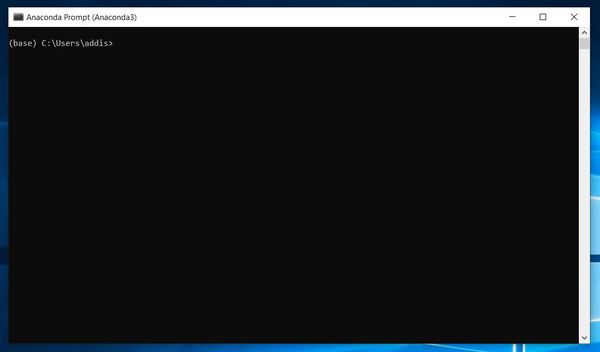
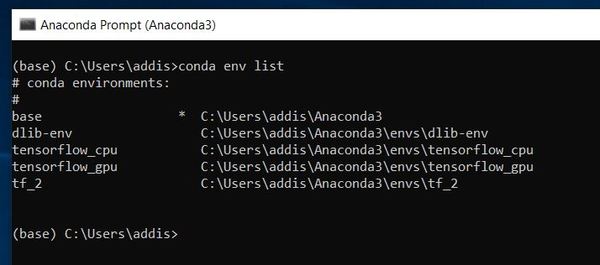
If you run your Python programs using Anaconda, open the Anaconda prompt.
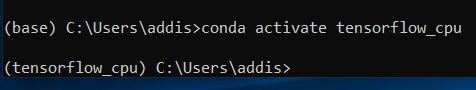
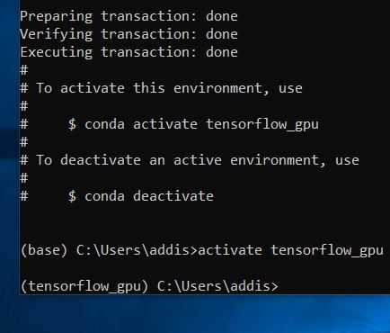
If you like to run your programs in a virtual environment, activate the virtual environment. I have a virtual environment named tf_2.
conda activate tf_2Navigate to the folder where you saved the Python program.
cd [path to folder]For example,
cd C:\MyFilesInstall any libraries that you need. I didn’t have some of the libraries in the “import” section of my code installed, so I’ll install them now.
pip install pandas
pip install seaborn
To run the code, type:
python vehicle_fuel_economy.py
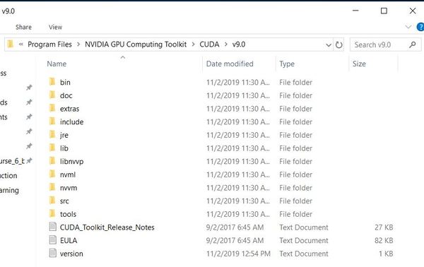
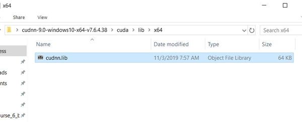
If you’re using a GPU with Tensorflow, and you’re getting error messages about libraries missing, go to this folder C:\Program Files\NVIDIA GPU Computing Toolkit\CUDA\v11.1\bin, and you can search on the Internet for the missing dll files. Download them, and then put them in that bin folder.
Code Output
In this section, I will pull out snippets of the code and show you the resulting output when you uncomment those lines.
  # Check the data set
  print("Original Data Set Excerpt")
  print(originalData.head())
  print()
  # Count how many NAs each data attribute has
  print("Number of NAs in the data set")
  print(data.isna().sum())
  print()
  # See a summary of the neural network
  # The first layer has 640 parameters
    #(9 input values * 64 neurons) + 64 bias values
  # The second layer has 4160 parameters
    #(64 input values * 64 neurons) + 64 bias values
  # The output layer has 65 parameters
    #(64 input values * 1 neuron) + 1 bias value
  print(neuralNet.summary())
  # Plot the neural network metrics (Training error and validation error)
  # Training error is the error when the trained neural network is
  #   run on the training data.
  # Validation error is used to minimize overfitting. It indicates how
  #   well the data fits on data it hasn't been trained on.
  plotNeuralNetMetrics(history)
  # Plot metrics
  plotNeuralNetMetrics(history2)
print(f'\nMean Absolute Error on Test Data Set = {meanAbsoluteError} miles per gallon')

  # Plot the predicted MPG vs. the true MPG
  # testingLabelData are the true MPG values
  # testingDataPredictions are the predicted MPG values
  plotTestingDataPredictions(testingLabelData, testingDataPredictions)
  # Plot the prediction error distribution
  plotPredictionError(testingLabelData, testingDataPredictions)
  # Save the neural network in Hierarchical Data Format version 5 (HDF5) format
  neuralNet2.save('fuel_economy_prediction_nnet.h5')

  # Import the saved model
  neuralNet3 = keras.models.load_model('fuel_economy_prediction_nnet.h5')
References
Quinlan,R. (1993). Combining Instance-Based and Model-Based Learning. In Proceedings on the Tenth International Conference of Machine Learning, 236-243, University of Massachusetts, Amherst. Morgan Kaufmann.