In this post, I will show you how to install TensorFlow 2 on Windows 10. TensorFlow2 is a free software library used for machine learning applications. It comes integrated with Keras, a neural-network library written in Python. If you want to work with neural networks and deep learning, TensorFlow 2 should be your software of choice because of its popularity both in academia and in industry. Let’s get started!
Type the command below to create a virtual environment named tf_2 with the latest version of Python installed. A virtual environment is like an independent Python workspace which has its own set of libraries and Python version installed. For example, you might have a project that needs to run using an older version of Python, like Python 2.7. You might have another project that requires Python 3.7. You can create separate virtual environments for these projects.
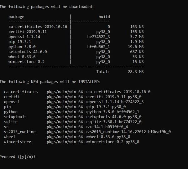
conda create -n tf_2 python
Press y and then ENTER.
Wait for the software to download.
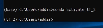
Once the download is finished, activate the virtual environment using this command:
conda activate tf_2
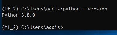
Check which version of Python you have installed on your system. I have Python 3.8.0.
python --version
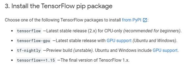
Choose a TensorFlow package. I’ll install TensorFlow CPU. Let’s type the following command:
pip install --upgrade tensorflow
You might see this error:
ERROR: Could not find a version that satisfies the requirement tensorflow (from versions: none)
ERROR: No matching distribution found for tensorflow
If you do, you need to downgrade your version of Python. TensorFlow is not yet compatible with your newest version of Python.
conda install python=3.6
Press y and then ENTER.
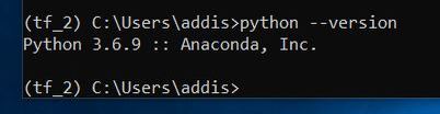
Check which version of Python you have installed on your system. I have Python 3.6.9 now.
python --version
Now install TensorFlow 2.
pip install --upgrade tensorflow
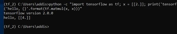
Wait for Tensorflow CPU to finish installing. Once it is finished installing, verify the installation by typing:
python -c "import tensorflow as tf; x = [[2.]]; print('tensorflow version', tf.__version__); print('hello, {}'.format(tf.matmul(x, x)))"
Here is the output:
You should see your TensorFlow version in the output.
You might see this message:
“I tensorflow/core/platform/cpu_feature_guard.cc:142] Your CPU supports instructions that this TensorFlow binary was not compiled to use: AVX2”
Don’t worry, TensorFlow is working just fine. To get rid of that message, you can set the environment variables inside the virtual environment. Type the following command:
set TF_CPP_MIN_LOG_LEVEL=2
Now run this command:
python -c "import tensorflow as tf; x = [[2.]]; print('tensorflow version', tf.__version__); print('hello, {}'.format(tf.matmul(x, x)))"
I’m now going to open up a text editor and type a Python program. I will save it to my D drive as fashion_mnist.py. Here is the code:
from __future__ import absolute_import, division, print_function, unicode_literals

# Import the key libraries
import matplotlib.pyplot as plt
import tensorflow as tf
import numpy as np

# Rename tf.keras.layers
layers = tf.keras.layers

# Print the TensorFlow version
print(tf.__version__)

# Load and prepare the MNIST dataset.
# Convert the samples from integers to floating-point numbers:
mnist = tf.keras.datasets.fashion_mnist
(x_train, y_train), (x_test, y_test) = mnist.load_data()
x_train, x_test = x_train / 255.0, x_test / 255.0

# Let's plot the data so we can see it
class_names = ['T-shirt/top', 'Trouser', 'Pullover', 'Dress', 'Coat', 'Sandal',
 'Shirt', 'Sneaker', 'Bag', 'Ankle boot']
plt.figure(figsize=(10,10))

for i in range(25):
 plt.subplot(5,5,i+1)
 plt.xticks([])
 plt.yticks([])
 plt.grid(False)
 plt.imshow(x_train[i], cmap=plt.cm.binary)
 plt.xlabel(class_names[y_train[i]])
plt.show()
Within your virtual environment in the Anaconda terminal, navigate to where you saved your code. I will type.
D:
Then:
cd D:\<YOUR_PATH>\install_tensorflow2
Type dir to see if the Python (.py) file is in that directory.
Now run the code:
python fashion_mnist.py
You should see this graphic pop up.
In the terminal window, press CTRL+C on your keyboard to stop the code from running.
Let’s add to our code. Open up the Python file again in the text editor and type the following code. If you are new to neural networks, don’t worry what everything means at this stage.
from __future__ import absolute_import, division, print_function, unicode_literals

# Import the key libraries
import matplotlib.pyplot as plt
import tensorflow as tf
import numpy as np

# Rename tf.keras.layers
layers = tf.keras.layers

# Print the TensorFlow version
print(tf.__version__)

# Load and prepare the MNIST dataset.
# Convert the samples from integers to floating-point numbers:
mnist = tf.keras.datasets.fashion_mnist
(x_train, y_train), (x_test, y_test) = mnist.load_data()
x_train, x_test = x_train / 255.0, x_test / 255.0

# Let's plot the data so we can see it
class_names = ['T-shirt/top', 'Trouser', 'Pullover', 'Dress', 'Coat', 'Sandal',
 'Shirt', 'Sneaker', 'Bag', 'Ankle boot']
plt.figure(figsize=(10,10))

for i in range(25):
 plt.subplot(5,5,i+1)
 plt.xticks([])
 plt.yticks([])
 plt.grid(False)
 plt.imshow(x_train[i], cmap=plt.cm.binary)
 plt.xlabel(class_names[y_train[i]])
plt.show()

# Build the neural network layer-by-layer
model = tf.keras.Sequential()
model.add(layers.Flatten()) # Make the input layer one-dimensional
model.add(layers.Dense(64, activation='relu')) # Layer has 64 nodes; Uses ReLU
model.add(layers.Dense(64, activation='relu')) # Layer has 64 nodes; Uses ReLU
model.add(layers.Dense(10, activation='softmax')) # Layer has 64 nodes; Uses Softmax

# Choose an optimizer and loss function for training:
model.compile(optimizer='adam',
 loss='sparse_categorical_crossentropy',
 metrics=['accuracy'])

# Train and evaluate the model's accuracy
model.fit(x_train, y_train, epochs=5)
model.evaluate(x_test,  y_test, verbose=2)
Run the code:
python fashion_mnist.py
When you see the plot of the clothes appear, just close that window so that the neural network build and run.
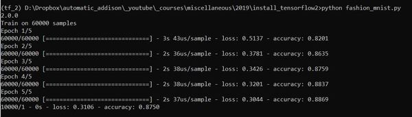
Here is the output.
The accuracy of classifying the clothing items was 87.5%. Pretty cool huh! Congratulations! You’ve built and run your first neural network on TensorFlow 2.
To deactivate the virtual environment, type:
conda deactivate
Then to exit the terminal, type:
exit
At this stage, I encourage you to go through the TensorFlow tutorials to get more practice using this really powerful tool.
The performance of reinforcement learning can be improved by incorporating supervised learning techniques. Let us take a look at a concrete example.
You all might be familiar with the Roomba robot created by iRobot. The Roomba robot is perhaps the most popular robot vacuum sold in the United States.
The Roomba is completely autonomous, moving around the room with ease, cleaning up dust, pet hair, and dirt along the way. In order to do its job, the Roomba contains a number of sensors that enable it to perceive the current state of the environment (i.e. your house).
Let us suppose that the Roomba is governed by a reinforcement learning policy. This learning policy could be improved if we have accurate readings of the current state of the environment. And one way to improve these readings is to incorporate computer vision.
Since reinforcement learning depends heavily on accurate readings of the current state of the environment, we could use deep neural networks (a supervised learning technique) to pre-train the robot so that it can perform common computer vision tasks such as recognizing objects, localizing objects, and classifying objects before we even start running the reinforcement learning algorithm. These “readings” would improve the state portion of the reinforcement learning loop.
Deep neural networks have already displayed remarkable accuracy for computer vision problems. We can use these techniques to enable the robot to get a more accurate reading of the current state of the environment so that it can then take the most appropriate actions towards maximizing cumulative reward.
In this post, I will walk you through how to build an artificial feedforward neural network trained with backpropagation, step-by-step. We will not use any fancy machine learning libraries, only basic Python libraries like Pandas and Numpy.
Our end goal is to evaluate the performance of an artificial feedforward neural network trained with backpropagation and to compare the performance using no hidden layers, one hidden layer, and two hidden layers. Five different data sets from the UCI Machine Learning Repository are used to compare performance: Breast Cancer, Glass, Iris, Soybean (small), and Vote.
We will use our neural network to do the following:
Predict if someone has breast cancer
Identify glass type
Identify flower species
Determine soybean disease type
Classify a representative as either a Democrat or Republican based on their voting patterns
I hypothesize that the neural networks with no hidden layers will outperform the networks with two hidden layers. My hypothesis is based on the notion that the simplest solutions are often the best solutions (i.e. Occam’s Razor).
What is an Artificial Feedforward Neural Network Trained with Backpropagation?
Background
An artificial feed-forward neural network (also known as multilayer perceptron) trained with backpropagation is an old machine learning technique that was developed in order to have machines that can mimic the brain. Neural networks were the focus of a lot of machine learning research during the 1980s and early 1990s but declined in popularity during the late 1990s.
Since 2010, neural networks have experienced a resurgence in popularity due to improvements in computing speed and the availability of massive amounts of data with which to train large-scale neural networks. In the real world, neural networks have been used to recognize speech, caption images, and even help self-driving cars learn how to park autonomously.
The Brain as Inspiration for Artificial Neural Networks
In
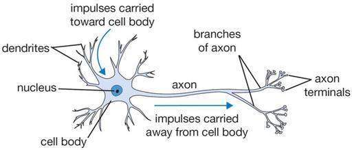
order to understand neural networks, it helps to first take a look at the basic
architecture of the human brain. The brain has 1011 neurons (Alpaydin,
2014). Neurons
are cells inside the brain that process information.
Each neuron contains a number of input wires called dendrites. Each neuron also has one output wire called an axon. The axon is used to send messages to other neurons. The axon of a sending neuron is connected to the dendrites of the receiving neuron via a synapse.
So,
in short, a neuron receives inputs from dendrites, performs a computation, and
sends the output to other neurons via the axon. This process is how information
flows through the brain. The messages sent between neurons are in the form of
electric pulses.
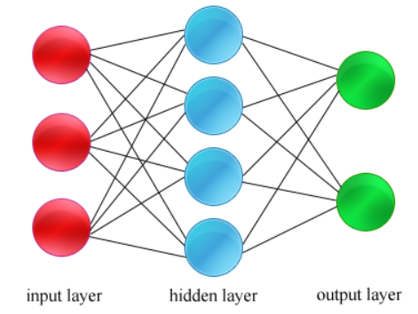
An
artificial neural network, the one used in machine learning, is a simplified
model of the actual human neural network explained above. It is typically
composed of zero or more layers.
Each
layer of the neural network is made up of nodes (analogous to neurons in the
brain). Nodes of one layer are connected to nodes in another layer by
connection weights, which are typically just floating-point numbers (e.g.
0.23342341). These numbers represent the strength of the connection between two
nodes.
The
job of a node in a hidden layer is to:
Receive
input values from each node in a preceding layer
Compute
a weighted sum of those input values
Send
that weighted sum through some activation function (e.g. logistic sigmoid
function or hyperbolic tangent function)
Send
the result of the computation in #3 to each node in the next layer of the
neural network.
Thus,
the output from the nodes in a given layer becomes the input for all nodes in the
next layer.
The
output layer of a network does steps 1-3 above. However, the result of the
computation from step #3 is a class prediction instead of an input to another
layer (since the output layer is the final layer).
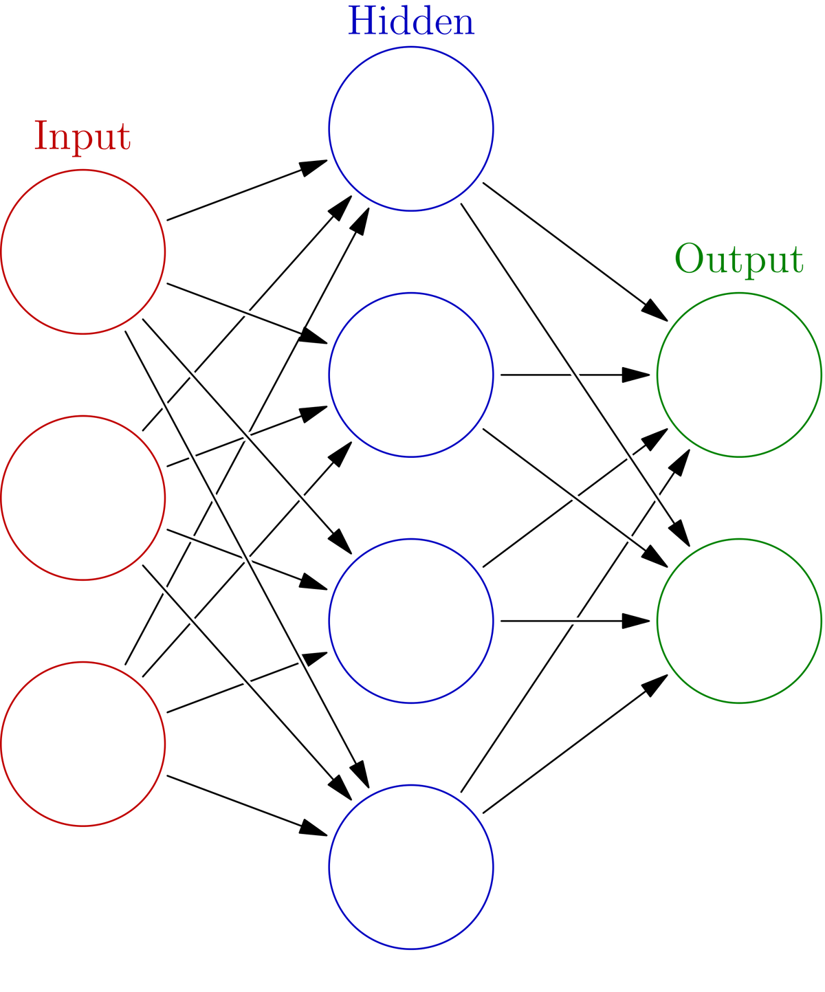
Here is a diagram of the process I explained above:
b stands for the bias term. This is a constant. It is like the b in the equation for a line, y = mx + b. It enables the model to have flexibility because, without that bias term, you cannot as easily adapt the weighted sum of inputs (i.e. mx) to fit the data (i.e. in the example of a simple line, the line cannot move up and down the y-axis without that b term).
w in the diagram above stands for the weights, and x stands for the input values.
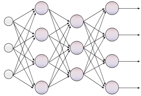
Here is a similar diagram, but now it is a two-layer neural network instead of single layer.
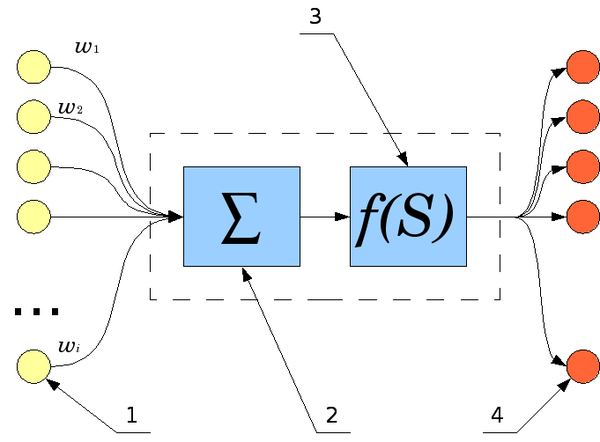
And here is one last way to look at the same thing I explained above:
Note that the yellow circles on the left represent the input values. w represents the weights. The sigma inside the box means that we calculated the weighted sum of the input values. We run that through the activation function f(S)…e.g. sigmoid function. And then out of that, pops the output, which is passed on to the nodes in the following layer.
Neural networks that contain many layers, for example more than 100, are called deep neural networks. Deep neural networks are the cornerstone of the rapidly growing field known as deep learning.
Training Phase
The objective during the training phase of a neural network is to determine all the connection weights. At the start of training, the weights of the network are initialized to small random values close to 0. After this step, training proceeds to the two main phases of the algorithm: forward propagation and backpropagation.
Forward Propagation
During
the forward propagation phase of a neural network, we process one instance (i.e.
one set of inputs) at a time. Hidden layers extract important features
contained in the input data by computing a weighted sum of the inputs and
running the result through the logistic sigmoid activation function. This
output relays to nodes in the next hidden layer where the data is transformed
yet again. This process continues until the data reaches the output layer.
The
output of the output layer is a predicted class value, which in this project is
a one-hot encoded class prediction vector. The index of the vector corresponds
to each class. For example, if a 1 is in the 0 index of the vector (and a 0 is in
all other indices of the vector), the class prediction is class 0. Because we
are dealing with 0s and 1s, the output vector can also be considered the
probability that an instance is in a given class.
Backpropagation
After
the input signal produced by a training instance propagates through the network
one layer at a time to the output layer, the backpropagation phase commences.
An error value is calculated at the output layer. This error corresponds to the
difference between the class predicted by the network and the actual (i.e.
true) class of the training instance.
The
prediction error is then propagated backward from the output layer to the input
layer. Blame for the error is assigned to each node in each layer, and then the
weights of each node of the neural network are updated accordingly (with the
goal to make more accurate class predictions for the next instance that flows
through the neural network) using stochastic gradient descent for the weight
optimization procedure.
Note
that weights of the neural network are adjusted on a training instance by
training instance basis. This online learning method is the preferred one for
classification problems of large size (Ĭordanov
& Jain, 2013).
The
forward propagation and backpropagation phases continue for a certain number of
epochs. A single epoch finishes when each training instance has been processed
exactly once.
Testing Phase
Once the neural network has been trained, it can be used to make predictions on new, unseen test instances. Test instances flow through the network one-by-one, and the resulting output (which is a vector of class probabilities) determines the classification.
Helpful Video
Below is a helpful video by Andrew Ng, a professor at Stanford University, that explains neural networks and is helpful for getting your head around the math. The video gets pretty complicated in some spots (esp. where he starts writing all sorts of mathematical notation and derivatives). My advice is to lookup anything that he explains that isn’t clear. Take it slow as you are learning about neural networks. There is no rush. This stuff isn’t easy to understand on your first encounter with it. Over time, the fog will begin to lift, and you will be able to understand how it all works.
Required Data Set Format for Feedforward Neural Network Trained with Backpropagation
Columns (0 through N)
0: Instance ID
1: Attribute 1
2: Attribute 2
3: Attribute 3
…
N: Actual Class
The program then adds two
additional columns for the testing set.
N + 1: Predicted Class
N + 2: Prediction Correct? (1 if yes, 0 if no)
Breast Cancer Data Set
This breast cancer data set
contains 699 instances, 10 attributes, and a class – malignant or benign (Wolberg,
1992).
Modification of Attribute Values
The actual class value was changed to “Benign”
or “Malignant.”
Attribute values were normalized to be in the
range 0 to 1.
Class values were vectorized using one-hot
encoding.
Missing Data
There were 16 missing attribute values, each denoted with a “?”. I
chose a random number between 1 and 10 (inclusive) to fill in the data.
Glass Data Set
This glass data set contains 214
instances, 10 attributes, and 7 classes (German, 1987). The purpose of the data set is to
identify the type of glass.
Modification of Attribute Values
Attribute values were normalized to be in the
range 0 to 1.
Class values were vectorized using one-hot
encoding.
Missing Data
There are no missing values in this data set.
Iris Data Set
This data set contains 3 classes
of 50 instances each (150 instances in total), where each class refers to a
different type of iris plant (Fisher, 1988).
Modification of Attribute Values
Attribute values were normalized to be in the
range 0 to 1.
Class values were vectorized using one-hot
encoding.
Missing Data
There were no missing attribute values.
Soybean Data Set (small)
This soybean (small) data set
contains 47 instances, 35 attributes, and 4 classes (Michalski, 1980). The purpose of the data set is to
determine the disease type.
Modification of Attribute Values
Attribute values were normalized to be in the
range 0 to 1.
Class values were vectorized using one-hot
encoding.
Attribute values that were all the same value were
removed.
Missing Data
There are no missing values in this data set.
Vote Data Set
This data set includes votes for
each of the U.S. House of Representatives Congressmen (435 instances) on the 16
key votes identified by the Congressional Quarterly Almanac (Schlimmer, 1987). The purpose of the data set is to identify
the representative as either a Democrat or Republican.
267 Democrats
168 Republicans
Modification of Attribute Values
I did the following modifications:
Changed all “y” to 1 and all “n” to 0.
Class values were vectorized using one-hot
encoding.
Missing Data
Missing values were denoted as “?”. To fill in
those missing values, I chose random number, either 0 (“No”) or 1 (“Yes”).
Stochastic Gradient Descent
I used stochastic gradient descent for optimizing the
weights.
In normal gradient descent, we need
to calculate the partial derivative of the cost function with respect to each
weight. For each partial derivative, we have to tally up the terms for each training
instance to compute the partial derivative of the cost function with respect to
that weight. What this means is that, if we have a lot of attributes and a
large dataset, gradient descent is slow. For this reason, stochastic gradient
descent was chosen since weights are updated after each training instance (as
opposed to after all training instances).
Here is a good video that explains stochastic gradient descent.
Some tuning was performed in this
project. The learning rate was set to 0.1, which was different than the 0.01
value that is often used for multi-layer feedforward neural networks (Montavon, 2012). Lower values resulted in much
longer training times and did not result in large improvements in
classification accuracy.
Epochs
The number of epochs chosen for
the main runs of the algorithm on the data sets was chosen to be 1000. Other
values were tested, but the number of epochs did not have a large impact on classification
accuracy.
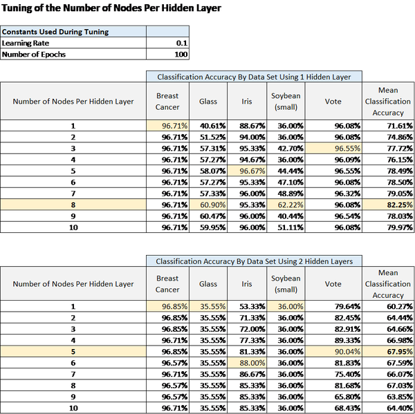
Number of Nodes per Hidden Layer
In order to tune the number of
nodes per hidden layer, I used a constant learning rate and constant number of
epochs. I then calculated the classification accuracy for each data set for a
set number of nodes per hidden layer. I performed this process using networks
with one hidden layer and networks with two hidden layers. The results of this
tuning process are below.
Note that the mean classification
accuracy across all data sets when one hidden layer was used for the neural
network reached a peak at eight nodes per hidden layer. This value of eight nodes
per hidden layer was used for the actual runs on the data sets.
For two hidden layers, the peak
mean classification accuracy was attained at five nodes per hidden layer. Thus,
when the algorithm was run on the data sets for two hidden layers, I used five
nodes per hidden layer for each data set to compare the classification accuracy
across the data sets.
Here is the full code for the neural network. This is all you need to run the program:
import pandas as pd # Import Pandas library
import numpy as np # Import Numpy library
from random import shuffle # Import shuffle() method from the random module
from random import seed # Import seed() method from the random module
from random import random # Import random() method from the random module
from collections import Counter # Used for counting
from math import exp # Import exp() function from the math module

# File name: neural_network.py
# Author: Addison Sears-Collins
# Date created: 7/30/2019
# Python version: 3.7
# Description: An artificial feedforward neural network trained
#   with backpropagation (also called multilayer perceptron)

# Required Data Set Format
# Columns (0 through N)
# 0: Attribute 0
# 1: Attribute 1
# 2: Attribute 2
# 3: Attribute 3
# ...
# N: Actual Class

# 2 additional columns are added for the test set.
# N + 1: Predicted Class
# N + 2: Prediction Correct?

ALGORITHM_NAME = "Feedforward Neural Network With Backpropagation"
SEPARATOR = ","  # Separator for the data set (e.g. "\t" for tab data)

def normalize(dataset):
    """
    Normalize the attribute values so that they are between 0 and 1, inclusive
    :param pandas_dataframe dataset: The original dataset as a Pandas dataframe
    :return: normalized_dataset
    :rtype: Pandas dataframe
    """
    # Generate a list of the column names
    column_names = list(dataset)

    # For every column except the actual class column
    for col in range(0, len(column_names) - 1):
        temp = dataset[column_names[col]] # Go column by column
        minimum = temp.min() # Get the minimum of the column
        maximum = temp.max() # Get the maximum of the column

        # Normalized all values in the column so that they
        # are between 0 and 1.
        # x_norm = (x_i - min(x))/(max(x) - min(x))
        dataset[column_names[col]] = dataset[column_names[col]] - minimum
        dataset[column_names[col]] = dataset[column_names[col]] / (
            maximum - minimum)

    normalized_dataset = dataset

    return normalized_dataset

def get_five_stratified_folds(dataset):
    """
    Implementation of five-fold stratified cross-validation. Divide the data
    set into five random folds. Make sure that the proportion of each class
    in each fold is roughly equal to its proportion in the entire data set.
    :param pandas_dataframe dataset: The original dataset as a Pandas dataframe
    :return: five_folds
    :rtype: list of folds where each fold is a list of instances(i.e. examples)
    """
    # Create five empty folds
    five_folds = list()
    fold0 = list()
    fold1 = list()
    fold2 = list()
    fold3 = list()
    fold4 = list()

    # Get the number of columns in the data set
    class_column = len(dataset[0]) - 1

    # Shuffle the data randomly
    shuffle(dataset)

    # Generate a list of the unique class values and their counts
    classes = list()  # Create an empty list named 'classes'

    # For each instance in the dataset, append the value of the class
    # to the end of the classes list
    for instance in dataset:
        classes.append(instance[class_column])

    # Create a list of the unique classes
    unique_classes = list(Counter(classes).keys())

    # For each unique class in the unique class list
    for uniqueclass in unique_classes:

        # Initialize the counter to 0
        counter = 0

        # Go through each instance of the data set and find instances that
        # are part of this unique class. Distribute them among one
        # of five folds
        for instance in dataset:

            # If we have a match
            if uniqueclass == instance[class_column]:

                # Allocate instance to fold0
                if counter == 0:

                    # Append this instance to the fold
                    fold0.append(instance)

                    # Increase the counter by 1
                    counter += 1

                # Allocate instance to fold1
                elif counter == 1:

                    # Append this instance to the fold
                    fold1.append(instance)

                    # Increase the counter by 1
                    counter += 1

                # Allocate instance to fold2
                elif counter == 2:

                    # Append this instance to the fold
                    fold2.append(instance)

                    # Increase the counter by 1
                    counter += 1

                # Allocate instance to fold3
                elif counter == 3:

                    # Append this instance to the fold
                    fold3.append(instance)

                    # Increase the counter by 1
                    counter += 1

                # Allocate instance to fold4
                else:

                    # Append this instance to the fold
                    fold4.append(instance)

                    # Reset the counter to 0
                    counter = 0

    # Shuffle the folds
    shuffle(fold0)
    shuffle(fold1)
    shuffle(fold2)
    shuffle(fold3)
    shuffle(fold4)

    # Add the five stratified folds to the list
    five_folds.append(fold0)
    five_folds.append(fold1)
    five_folds.append(fold2)
    five_folds.append(fold3)
    five_folds.append(fold4)

    return five_folds

def initialize_neural_net(
    no_inputs, no_hidden_layers, no_nodes_per_hidden_layer, no_outputs):
    """
    Generates a new neural network that is ready to be trained.
    Network (list of layers): 0+ hidden layers, and output layer
    Input Layer (list of attribute values): A row from the training set
    Hidden Layer (list of dictionaries): A set of nodes (i.e. neurons)
    Output Layer (list of dictionaries): A set of nodes, one node per class
    Node (dictionary): Contains a set of weights, one weight for each input
      to the layer containing that node + an additional weight for the bias.
      Each node is represented as a dictionary that stores key-value pairs
      Each key corresponds to a property of that node (e.g. weights).
      Weights will be initialized to small random values between 0 and 1.
    :param int no_inputs: Numper of inputs (i.e. attributes)
    :param int no_hidden_layers: Numper of hidden layers (0 or more)
    :param int no_nodes_per_hidden_layer: Numper of nodes per hidden layer
    :param int no_outputs: Numper of outputs (one output node per class)
    :return: network
    :rtype:list (i.e. list of layers: hidden layers, output layer)
    """

    # Create an empty list
    network = list()

    # Create the the hidden layers
    hidden_layer = list()
    hl_counter = 0

    # Create the output layer
    output_layer = list()

    # If this neural network contains hidden layers
    if no_hidden_layers > 0:

        # Build one hidden layer at a time
        for layer in range(no_hidden_layers):

            # Reset to an empty hidden layer
            hidden_layer = list()

            # If this is the first hidden layer
            if hl_counter == 0:

                # Build one node at a time
                for node in range(no_nodes_per_hidden_layer):

                    initial_weights = list()

                    # Each node in the hidden layer has no_inputs + 1 weights,
                    # initialized to a random number in the range [0.0, 1.0)
                    for i in range(no_inputs + 1):
                        initial_weights.append(random())

                    # Add the node to the first hidden layer
                    hidden_layer.append({'weights':initial_weights})

                # Finished building the first hidden layer
                hl_counter += 1

                # Add this first hidden layer to the front of the neural
                # network
                network.append(hidden_layer)

            # If this is not the first hidden layer
            else:

                # Build one node at a time
                for node in range(no_nodes_per_hidden_layer):

                    initial_weights = list()

                    # Each node in the hidden layer has
                    # no_nodes_per_hidden_layer + 1 weights, initialized to
                    # a random number in the range [0.0, 1.0)
                    for i in range(no_nodes_per_hidden_layer + 1):
                        initial_weights.append(random())

                    hidden_layer.append({'weights':initial_weights})

                # Add this newly built hidden layer to the neural network
                network.append(hidden_layer)

        # Build the output layer
        for outputnode in range(no_outputs):

            initial_weights = list()

            # Each node in the output layer has no_nodes_per_hidden_layer
            # + 1 weights, initialized to a random number in
            # the range [0.0, 1.0)
            for i in range(no_nodes_per_hidden_layer + 1):
                initial_weights.append(random())

            # Add this output node to the output layer
            output_layer.append({'weights':initial_weights})

        # Add the output layer to the neural network
        network.append(output_layer)

    # A neural network has no hidden layers
    else:

        # Build the output layer
        for outputnode in range(no_outputs):

            initial_weights = list()

            # Each node in the hidden layer has no_inputs + 1 weights,
            # initialized to a random number in the range [0.0, 1.0)
            for i in range(no_inputs + 1):
                initial_weights.append(random())

            # Add this output node to the output layer
            output_layer.append({'weights':initial_weights})

        network.append(output_layer)

    # Finished building the initial neural network
    return network

def weighted_sum_of_inputs(weights, inputs):
    """
    Calculates the weighted sum of inputs plus the bias
    :param list weights: A list of weights. Each node has a list of weights.
    :param list inputs: A list of input values. These can be a single row
        of attribute values or the output from nodes from the previous layer
    :return: weighted_sum
    :rtype: float
    """
    # We assume that the last weight is the bias value
    # The bias value is a special weight that does not multiply with an input
    # value (or we could assume its corresponding input value is always 1)
    # The bias is similar to the intercept constant b in y = mx + b. It enables
    # a (e.g. sigmoid) curve to be shifted to create a better fit
    # to the data. Without the bias term b, the line always goes through the
    # origin (0,0) and cannot adapt as well to the data.
    # In y = mx + b, we assume b * x_0 where x_0 = 1

    # Initiate the weighted sum with the bias term. Assume the last weight is
    # the bias term
    weighted_sum = weights[-1]

    for index in range(len(weights) - 1):
        weighted_sum += weights[index] * inputs[index]

    return weighted_sum

def sigmoid(weighted_sum_of_inputs_plus_bias):
    """
    Run the weighted sum of the inputs + bias through
    the sigmoid activation function.
    :param float weighted_sum_of_inputs_plus_bias: Node summation term
    :return: sigmoid(weighted_sum_of_inputs_plus_bias)
    """
    return 1.0 / (1.0 + exp(-weighted_sum_of_inputs_plus_bias))

def forward_propagate(network, instance):
    """
    Instances move forward through the neural network from one layer
    to the next layer. At each layer, the outputs are calculated for each
    node. These outputs are the inputs for the nodes in the next layer.
    The last set of outputs is the output for the nodes in the output
    layer.
    :param list network: List of layers: 0+ hidden layers, 1 output layer
    :param list instance (a single training/test instance from the data set)
    :return: outputs
    :rtype: list
    """
    inputs = instance

    # For each layer in the neural network
    for layer in network:

        # These will store the outputs for this layer
        new_inputs = list()

        # For each node in this layer
        for node in layer:

            # Calculate the weighted sum + bias term
            weighted_sum = weighted_sum_of_inputs(node['weights'], inputs)

            # Run the weighted sum through the activation function
            # and store the result in this node's dictionary.
            # Now the node's dictionary has two keys, weights and output.
            node['output'] = sigmoid(weighted_sum)

            # Used for debugging
            #print(node)

            # Add the output of the node to the new_inputs list
            new_inputs.append(node['output'])

        # Update the inputs list
        inputs = new_inputs

    # We have reached the output layer
    outputs = inputs

    return outputs

def sigmoid_derivative(output):
    """
    The derivative of the sigmoid activation function with respect
    to the weighted summation term of the node.
    Formally (after a lot of calculus), this derivative is:
        derivative = sigmoid(weighted_sum_of_inputs_plus_bias) *
        (1 - sigmoid(weighted_sum_of_inputs_plus_bias))
                   = node_ouput * (1 - node_output)
    This method is used during the backpropagation phase.
    :param list output: Output of a node (generated during the forward
        propagation phase)
    :return: sigmoid_der
    :rtype: float
    """
    return output * (1.0 - output)

def back_propagate(network, actual):
    """
    In backpropagation, the error is computed between the predicted output by
    the network and the actual output as determined by the data set. This error
    propagates backwards from the output layer to the first hidden layer. The
    weights in each layer are updated along the way in response to the error.
    The goal is to reduce the prediction error for the next training instance
    that forward propagates through the network.
    :param network list: The neural network
    :param actual list: A list of the actual output from the data set
    """
    # Iterate in reverse order (i.e. starts from the output layer)
    for i in reversed(range(len(network))):

        # Work one layer at a time
        layer = network[i]

        # Keep track of the errors for the nodes in this layer
        errors = list()

        # If this is a hidden layer
        if i != len(network) - 1:

            # For each node_j in this hidden layer
            for j in range(len(layer)):

                # Reset the error value
                error = 0.0

                # Calculate the weighted error.
                # The error values come from the error (i.e. delta) calculated
                # at each node in the layer just to the "right" of this layer.
                # This error is weighted by the weight connections between the
                # node in this hidden layer and the nodes in the layer just
                # to the "right" of this layer.
                for node in network[i + 1]:
                    error += (node['weights'][j] * node['delta'])

                # Add the weighted error for node_j to the
                # errors list
                errors.append(error)

        # If this is the output layer
        else:

            # For each node in the output layer
            for j in range(len(layer)):

                # Store this node (i.e. dictionary)
                node = layer[j]

                # Actual - Predicted = Error
                errors.append(actual[j] - node['output'])

        # Calculate the delta for each node_j in this layer
        for j in range(len(layer)):
            node = layer[j]

            # Add an item to the node's dictionary with the
            # key as delta.
            node['delta'] = errors[j] * sigmoid_derivative(node['output'])

def update_weights(network, instance, learning_rate):
    """
    After the deltas (errors) have been calculated for each node in
    each layer of the neural network, the weights can be updated.
    new_weight = old_weight + learning_rate * delta * input_value
    :param list network: List of layers: 0+ hidden layers, 1 output layer
    :param list instance: A single training/test instance from the data set
    :param float learning_rate: Controls step size in the stochastic gradient
        descent procedure.
    """
    # For each layer in the network
    for layer_index in range(len(network)):

        # Extract all the attribute values, excluding the class value
        inputs = instance[:-1]

        # If this is not the first hidden layer
        if layer_index != 0:

            # Go through each node in the previous layer and add extract the
            # output from that node. The output from the previous layer
            # is the input to this layer.
            inputs = [node['output'] for node in network[layer_index - 1]]

        # For each node in this layer
        for node in network[layer_index]:

            # Go through each input value
            for j in range(len(inputs)):

                # Update the weights
                node['weights'][j] += learning_rate * node['delta'] * inputs[j]

            # Updating the bias weight
            node['weights'][-1] += learning_rate * node['delta']

def train_neural_net(
    network, training_set, learning_rate, no_epochs, no_outputs):
    """
    Train a neural network that has already been initialized.
    Training is done using stochastic gradient descent where the weights
    are updated one training instance at a time rather than after the
    entire training set (as is the case with gradient descent).
    :param list network: The neural network, which is a list of layers
    :param list training_set: A list of training instances (i.e. examples)
    :param float learning_rate: Controls step size of gradient descent
    :param int no_epochs: How many passes we will make through training set
    :param int no_outputs: The number of output nodes (equal to # of classes)
    """
    # Go through the entire training set a fixed number of times (i.e. epochs)
    for epoch in range(no_epochs):

        # Update the weights one instance at a time
        for instance in training_set:

            # Forward propagate the training instance through the network
            # and produce the output, which is a list.
            outputs = forward_propagate(network, instance)

            # Vectorize the output using one hot encoding.
            # Create a list called actual_output that is the same length
            # as the number of outputs. Put a 1 in the place of the actual
            # class.
            actual_output = [0 for i in range(no_outputs)]
            actual_output[int(instance[-1])] = 1

            back_propagate(network, actual_output)
            update_weights(network, instance, learning_rate)

def predict_class(network, instance):
    """
    Make a class prediction given a trained neural network and
    an instance from the test data set.
    :param list network: The neural network, which is a list of layers
    :param list instance: A single training/test instance from the data set
    :return class_prediction
    :rtype int
    """
    outputs = forward_propagate(network, instance)

    # Return the index that has the highest probability. This index
    # is the class value. Assume class values begin at 0 and go
    # upwards by 1 (i.e. 0, 1, 2, ...)
    class_prediction = outputs.index(max(outputs))

    return class_prediction

def calculate_accuracy(actual, predicted):
    """
    Calculates the accuracy percentages
    :param list actual: Actual class values
    :param list predicted: predicted class values
    :return: classification_accuracy
    :rtype: float (as a percentage)
    """
    number_of_correct_predictions = 0
    for index in range(len(actual)):
        if actual[index] == predicted[index]:
            number_of_correct_predictions += 1

    classification_accuracy = (
        number_of_correct_predictions / float(len(actual))) * 100.0
    return classification_accuracy

def get_test_set_predictions(
    training_set, test_set, learning_rate, no_epochs,
    no_hidden_layers, no_nodes_per_hidden_layer):
    """
    This method is the workhorse.
    A new neutal network is initialized.
    The network is trained on the training set.
    The trained neural network is used to generate predictions on the
    test data set.
    :param list training_set
    :param list test_set
    :param float learning_rate
    :param int no_epochs
    :param int no_hidden_layers
    :param int no_nodes_per_hidden_layer
    :return network, class_predictions
    :rtype list, list
    """
    # Get the number of attribute values
    no_inputs = len(training_set[0]) - 1

    # Calculate the number of unique classes
    no_outputs = len(set([instance[-1] for instance in training_set]))

    # Build a new neural network
    network = initialize_neural_net(
        no_inputs, no_hidden_layers, no_nodes_per_hidden_layer, no_outputs)

    train_neural_net(
        network, training_set, learning_rate, no_epochs, no_outputs)

    # Store the class predictions for each test instance
    class_predictions = list()
    for instance in test_set:
        cl_prediction = predict_class(network, instance)
        class_predictions.append(cl_prediction)

    # Return the learned model as well as the class predictions
    return network, class_predictions

###############################################################

def main():
    """
    The main method of the program
    """
    LEARNING_RATE = 0.1 # Used for stochastic gradient descent procedure
    NO_EPOCHS = 1000 # Epoch is one complete pass through training data
    NO_HIDDEN_LAYERS = 1 # Number of hidden layers
    NO_NODES_PER_HIDDEN_LAYER = 8 # Number of nodes per hidden layer

    # Welcome message
    print("Welcome to the " +  ALGORITHM_NAME + " Program!")
    print()

    # Directory where data set is located
    #data_path = input("Enter the path to your input file: ")
    data_path = "vote.txt"

    # Read the full text file and store records in a Pandas dataframe
    pd_data_set = pd.read_csv(data_path, sep=SEPARATOR)

    # Show functioning of the program
    #trace_runs_file = input("Enter the name of your trace runs file: ")
    trace_runs_file = "vote_nn_trace_runs.txt"

    ## Open a new file to save trace runs
    outfile_tr = open(trace_runs_file,"w")

    # Testing statistics
    #test_stats_file = input("Enter the name of your test statistics file: ")
    test_stats_file = "vote_nn_test_stats.txt"

    ## Open a test_stats_file
    outfile_ts = open(test_stats_file,"w")

    # Generate a list of the column names
    column_names = list(pd_data_set)

    # The input layer in the neural network
    # will have one node for each attribute value
    no_of_inputs = len(column_names) - 1

    # Make a list of the unique classes
    list_of_unique_classes = pd.unique(pd_data_set["Actual Class"])

    # The output layer in the neural network
    # will have one node for each class value
    no_of_outputs = len(list_of_unique_classes)

    # Replace all the class values with numbers, starting from 0
    # in the Pandas dataframe.
    for cl in range(0, len(list_of_unique_classes)):
        pd_data_set["Actual Class"].replace(
            list_of_unique_classes[cl], cl ,inplace=True)

    # Normalize the attribute values so that they are all between 0
    # and 1, inclusive
    normalized_pd_data_set = normalize(pd_data_set)

    # Convert normalized Pandas dataframe into a list
    dataset_as_list = normalized_pd_data_set.values.tolist()

    # Set the seed for random number generator
    seed(1)

    # Get a list of 5 stratified folds because we are doing
    # five-fold stratified cross-validation
    fv_folds = get_five_stratified_folds(dataset_as_list)

    # Keep track of the scores for each of the five experiments
    scores = list()

    experiment_counter = 0
    for fold in fv_folds:

        print()
        print("Running Experiment " + str(experiment_counter) + " ...")
        print()
        outfile_tr.write("Running Experiment " + str(
            experiment_counter) + " ...\n")
        outfile_tr.write("\n")

        # Get all the folds and store them in the training set
        training_set = list(fv_folds)

        # Four folds make up the training set
        training_set.remove(fold)

        # Combined all the folds so that all we have is a list
        # of training instances
        training_set = sum(training_set, [])

        # Initialize a test set
        test_set = list()

        # For each instance in this test fold
        for instance in fold:

            # Create a copy and store it
            copy_of_instance = list(instance)
            test_set.append(copy_of_instance)

        # Get the trained neural network and the predicted values
        # for each test instance
        neural_net, predicted_values = get_test_set_predictions(
            training_set, test_set,LEARNING_RATE,NO_EPOCHS,
            NO_HIDDEN_LAYERS,NO_NODES_PER_HIDDEN_LAYER)
        actual_values = [instance[-1] for instance in fold]
        accuracy = calculate_accuracy(actual_values, predicted_values)
        scores.append(accuracy)

        # Print the learned model
        print("Experiment " + str(
            experiment_counter) + " Trained Neural Network")
        print()
        for layer in neural_net:
            print(layer)
        print()
        outfile_tr.write("Experiment " + str(
            experiment_counter) + " Trained Neural Network")
        outfile_tr.write("\n")
        outfile_tr.write("\n")
        for layer in neural_net:
            outfile_tr.write(str(layer))
            outfile_tr.write("\n")
        outfile_tr.write("\n\n")

        # Print the classifications on the test instances
        print("Experiment " + str(
            experiment_counter) + " Classifications on Test Instances")
        print()
        outfile_tr.write("Experiment " + str(
            experiment_counter) + " Classifications on Test Instances")
        outfile_tr.write("\n\n")
        test_df = pd.DataFrame(test_set, columns=column_names)

        # Add 2 additional columns to the testing dataframe
        test_df = test_df.reindex(
        columns=[*test_df.columns.tolist(
        ), 'Predicted Class', 'Prediction Correct?'])

        # Add the predicted values to the "Predicted Class" column
        # Indicate if the prediction was correct or not.
        for pre_val_index in range(len(predicted_values)):
            test_df.loc[pre_val_index, "Predicted Class"] = predicted_values[
                pre_val_index]
            if test_df.loc[pre_val_index, "Actual Class"] == test_df.loc[
                pre_val_index, "Predicted Class"]:
                test_df.loc[pre_val_index, "Prediction Correct?"] = "Yes"
            else:
                test_df.loc[pre_val_index, "Prediction Correct?"] = "No"

        # Replace all the class values with the name of the class
        for cl in range(0, len(list_of_unique_classes)):
            test_df["Actual Class"].replace(
                cl, list_of_unique_classes[cl] ,inplace=True)
            test_df["Predicted Class"].replace(
                cl, list_of_unique_classes[cl] ,inplace=True)

        # Print out the test data frame
        print(test_df)
        print()
        print()
        outfile_tr.write(str(test_df))
        outfile_tr.write("\n\n")

        # Go to the next experiment
        experiment_counter += 1

    print("Experiments Completed.\n")
    outfile_tr.write("Experiments Completed.\n\n")

    # Print the test stats
    print("------------------------------------------------------------------")
    print(ALGORITHM_NAME + " Summary Statistics")
    print("------------------------------------------------------------------")
    print("Data Set : " + data_path)
    print()
    print("Learning Rate: " + str(LEARNING_RATE))
    print("Number of Epochs: " + str(NO_EPOCHS))
    print("Number of Hidden Layers: " + str(NO_HIDDEN_LAYERS))
    print("Number of Nodes Per Hidden Layer: " + str(
        NO_NODES_PER_HIDDEN_LAYER))
    print()
    print("Accuracy Statistics for All 5 Experiments: %s" % scores)
    print()
    print()
    print("Classification Accuracy: %.3f%%" % (
        sum(scores)/float(len(scores))))

    outfile_ts.write(
        "------------------------------------------------------------------\n")
    outfile_ts.write(ALGORITHM_NAME + " Summary Statistics\n")
    outfile_ts.write(
        "------------------------------------------------------------------\n")
    outfile_ts.write("Data Set : " + data_path +"\n\n")
    outfile_ts.write("Learning Rate: " + str(LEARNING_RATE) + "\n")
    outfile_ts.write("Number of Epochs: " + str(NO_EPOCHS) + "\n")
    outfile_ts.write("Number of Hidden Layers: " + str(
        NO_HIDDEN_LAYERS) + "\n")
    outfile_ts.write("Number of Nodes Per Hidden Layer: " + str(
        NO_NODES_PER_HIDDEN_LAYER) + "\n")
    outfile_ts.write(
        "Accuracy Statistics for All 5 Experiments: %s" % str(scores))
    outfile_ts.write("\n\n")
    outfile_ts.write("Classification Accuracy: %.3f%%" % (
        sum(scores)/float(len(scores))))

    ## Close the files
    outfile_tr.close()
    outfile_ts.close()

main()
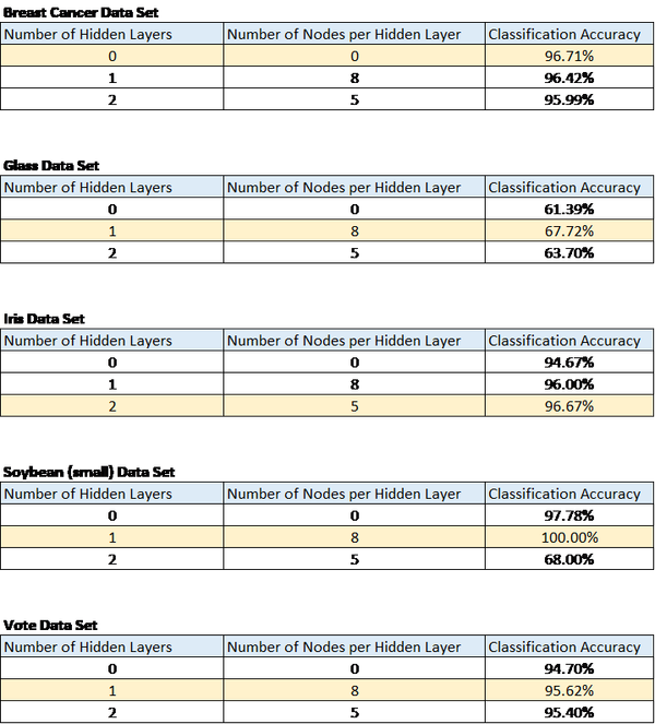
The breast cancer data set results
were in line with what I expected. The simpler model, the one with no hidden
layers, ended up generating the highest classification accuracy. Classification
accuracy was just short of 97%. In other words, the neural network that had no
hidden layers successfully classified a patient as either malignant or benign
with an almost 97% accuracy.
These results also suggest that
the amount of training data has a direct impact on performance. Higher amounts
of data (699 instances in this case) can lead to better learning and better
classification accuracy on new, unseen instances.
Glass Data Set
The performance of the neural
network on the glass data set was the worst out of all of the data sets. The
ability of the network to correctly identify the type of glass given the
attribute values never exceeded 70%.
I hypothesize that the poor
performance on the glass data set is due to the high numbers of classes
combined with a relatively smaller data set.
Iris Data Set
Classification accuracy was
superb on the iris dataset, attaining a classification accuracy around 97%. The
results of the iris dataset were surprising given that the more complicated
neural network with two hidden layers and five nodes per hidden layer outperformed
the simpler neural network that had no hidden layers. In this case, it appears
that the iris dataset benefited from the increasing layers of abstraction
provided by a higher number of layers.
Soybean Data Set (small)
Performance on the soybean data set
was stellar and was the highest of all of the data sets but also had the
largest standard deviation for the classification accuracy. Note that
classification accuracy reached a peak of 100% using one hidden layer and eight
nodes for the hidden layer. However, when I added an additional hidden layer,
classification accuracy dropped to under 70%.
The reason for the high standard
deviation of the classification accuracy is unclear, but I hypothesize it has
to do with the relatively small number of training instances. Future work would
need to be performed with the soybean large dataset available from the UCI Machine
Learning Repository to see if these results remain consistent.
The results of the soybean runs suggest
that large numbers of relevant attributes can help a machine learning algorithm
create more accurate classifications.
Vote Data Set
The vote data set did not yield the
stellar performance of the soybean data set, but classification accuracy was
still solid at ~96% using one hidden layer and eight nodes per hidden layer.
These results are in line with what I expected because voting behavior should
provide a powerful predictor of whether a candidate is a Democrat or
Republican. I would have been surprised had I observed classification
accuracies that were lower since members of Congress tend to vote along party
lines on most issues.
Summary and Conclusions
My hypothesis was incorrect. In
some cases, simple neural networks with no hidden layers outperformed more
complex neural networks with 1+ hidden layers. However, in other cases, more
complex neural networks with multiple hidden layers outperformed the network
with no hidden layers. The reason why some data is more amenable to networks
with hidden layers instead of without hidden layers is unclear.
Other conclusions include the
following:
Higher amounts of data can lead to better
learning and better classification accuracy on new, unseen instances.
Large numbers of relevant attributes can help a neural
network create more accurate classifications.
Neural networks are powerful and can achieve
excellent results on both binary and multi-class classification problems.
Alpaydin, E. (2014). Introduction to Machine
Learning. Cambridge, Massachusetts: The MIT Press.
Fisher, R. (1988, July 01). Iris Data Set.
Retrieved from Machine Learning Repository: https://archive.ics.uci.edu/ml/datasets/iris
German, B. (1987, September 1). Glass
Identification Data Set. Retrieved from UCI Machine Learning Repository:
https://archive.ics.uci.edu/ml/datasets/Glass+Identification
Ĭordanov, I., & Jain, L. C. (2013). Innovations
in Intelligent Machines –3 : Contemporary Achievements in Intelligent
Systems. Berlin: Springer.
Michalski, R. (1980). Learning by being told and
learning from examples: an experimental comparison of the two methodes of
knowledge acquisition in the context of developing an expert system for
soybean disease diagnosis. International Journal of Policy Analysis and
Information Systems, 4(2), 125-161.
Montavon, G. O. (2012). Neural Networks : Tricks
of the Trade. New York: Springer.
Schlimmer, J. (1987, 04 27). Congressional Voting
Records Data Set. Retrieved from Machine Learning Repository:
https://archive.ics.uci.edu/ml/datasets/Congressional+Voting+Records
Wolberg, W. (1992, 07 15). Breast Cancer Wisconsin
(Original) Data Set. Retrieved from Machine Learning Repository:
https://archive.ics.uci.edu/ml/datasets/Breast+Cancer+Wisconsin+%28Original%25