
We see incredible demos of robots doing backflips, but the reality is that some of the simplest human tasks remain impossible for machines.
In this video, I break down the 5 biggest unsolved problems in robotics, from dexterous manipulation to the economics.
The future of robotics isn’t about hype; it’s about solving these fundamental challenges.
Tag: ground
Autonomous Docking with AprilTags Using Nav2 – ROS 2 Jazzy
Precise docking is a key capability for autonomous mobile robots. While Nav2 excels at general path planning and obstacle avoidance, docking often requires more accurate position information than standard navigation provides. This is where AprilTags come in – they’re visual markers that help robots determine their exact position and orientation relative to a docking station.
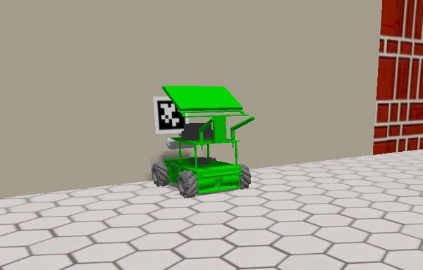
In this tutorial, we’ll implement automated docking by combining Nav2’s docking server with AprilTag detection. We’ll mount an AprilTag near our docking station and configure our robot to use it as a visual reference point. The Nav2 docking server will handle the approach and final alignment, using the AprilTag’s position data to guide the robot into the dock. Here is what you will be able to build by the end of this tutorial:
We’ll build this system in clear steps:
- Set up AprilTag detection to process our robot’s camera images
- Configure the Nav2 docking server to use AprilTag data
- Test our docking system in simulation
In this tutorial, we will implement AprilTag detection using ROS 2, giving you hands-on experience with an important technology in robot vision. We will use the CPU version of AprilTag detection from ROS 2. You can find a GPU-accelerated drop-in replacement for this CPU version here on the NVIDIA Isaac website.
Real-World Applications
AprilTags are used in many real-world situations. Here are some examples:
- Robotic Arms:
- Helping robotic arms in factories pick up parts from exact locations
- Guiding robotic arms in fast food restaurants, like those made by Miso Robotics, to assist with cooking tasks
- Mobile Robots:
- Helping delivery robots navigate through office buildings or hospitals
- Assisting mobile robots to dock precisely at battery charging stations
- Drones:
- Enabling drones to land accurately on specific locations marked with AprilTags
- Guiding drones for indoor inspections where GPS doesn’t work well
Prerequisites
- You have completed this tutorial: Getting Started With the Simple Commander API – ROS 2 Jazzy.
All my code for this project is located here on GitHub.
What Are AprilTags?
AprilTags are visual markers designed specifically for robotics and computer vision applications. These tags appear as small black and white squares with unique patterns inside. Their primary purpose is to help robots and cameras quickly determine their position and orientation in space.
When a robot’s camera spots an AprilTag, it can instantly calculate how far away the tag is, what angle it’s viewing the tag from, and which specific tag it’s looking at, as each tag has a unique identifier.
AprilTags offer several advantages:
- They’re inexpensive to produce and can be quickly printed on a plain sheet of white paper
- They perform well in various lighting conditions
- They allow for fast detection – an important feature for real-time applications.
Why Use AprilTags Instead of ArUco Markers?
You may have heard of another type of visual tag used in robotics called ArUco markers. ArUco markers are similar to AprilTags. They look like small black and white squares with patterns inside, much like AprilTags. However, AprilTags have some advantages:
- Better in Difficult Situations: AprilTags work better when lighting is not perfect or when part of the tag is hidden.
- More Accurate: AprilTags give robots a more precise idea of where they are, especially when far away or viewed at odd angles.
- Faster to Identify: Robots can usually find and read AprilTags more quickly than with ArUco markers, which is important when things need to happen fast.
- Fewer Mistakes: AprilTags are less likely to be confused with other objects or misread.
What Do We Need to Do?
Remember Automatic Addison’s 10 Ps of robotics: Prior Proper Planning Prevents Poor Performance. Poor Performance Promotes Pain.
Let’s begin with the end in mind and think through all the steps we need to take to get to our end goal, which is to have our robot dock to a docking station using the Nav2 Docking Server.
First, we need to add an AprilTag to our cafe world environment in Gazebo. This tag will serve as the visual marker for our robot’s docking station. The tag needs to be placed at a specific position and orientation that makes sense for docking.
Now open a new terminal window, and type the following command to launch the robot. Wait until Gazebo and RViz come fully up, which can take up to 30 seconds:
navor
bash ~/ros2_ws/src/yahboom_rosmaster/yahboom_rosmaster_bringup/scripts/rosmaster_x3_navigation.sh Type this command in the terminal window:
ros2 topic list | grep cam_1Our robot’s depth camera currently publishes raw images to /cam_1/color/image_raw as well as camera information to /cam_1/color/camera_info.
To see the image on /cam_1/color/image_raw, type:
sudo apt-get install ros-$ROS_DISTRO-image-viewThen run the image viewer:
ros2 run image_view image_view --ros-args -r image:=cam_1/color/image_rawYou can move your robot around the room.
For these raw camera images to be useful for AprilTag detection, we need to process them through a ROS 2 package called image_proc. We will use the rectify node to achieve this. This node:
Subscribes to:
- /cam_1/color/image_raw (sensor_msgs/msg/Image)
- /cam_1/color/camera_info (sensor_msgs/msg/CameraInfo)
Publishes:
- /cam_1/color/image_rect (sensor_msgs/msg/Image)
Why did we have to do this step? For AprilTag detection, we need rectified images, which remove camera lens distortion. The camera’s lens naturally bends the image a bit (like looking through a curved glass), which can make the square tags look slightly warped – rectification fixes this so the tags are easier to detect.
With our rectified images ready, we will use the CPU-based apriltag_ros package for detection. This node:
Subscribes to:
- /cam_1/color/image_rect (sensor_msgs/msg/Image)
- /cam_1/color/camera_info (sensor_msgs/msg/CameraInfo)
Publishes:
- /tf (tf2_msgs/msg/TFMessage)
- detections (apriltag_msgs/msg/AprilTagDetectionArray)
Alternatively, if you have an NVIDIA GPU, you could use Isaac ROS AprilTag. This node would:
Subscribe to:
- /cam_1/color/image_rect (sensor_msgs/msg/Image)
- /cam_1/color/camera_info (sensor_msgs/msg/CameraInfo)
Publish:
- tag_detections (isaac_ros_apriltag_interfaces/msg/AprilTagDetectionArray)
- tf (tf2_msgs/msg/TFMessage)
The Nav2 Docking Server uses these AprilTag detections through its SimpleChargingDock plugin. Looking at the SimpleChargingDock source code, this plugin specifically subscribes to:
- detected_dock_pose (geometry_msgs/msg/PoseStamped) – For getting the current pose of the dock
The complete pipeline works like this:
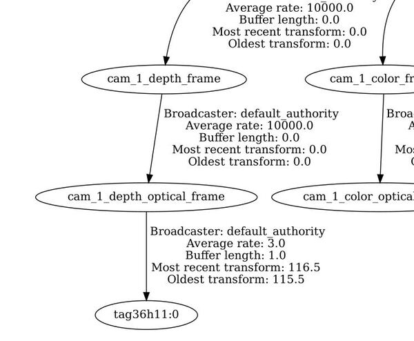
- apriltag_ros (or isaac_ros_apriltag) detects our tag (ID 0 from family 36h11) and publishes the transform:
- Parent frame: cam_1_depth_optical_frame (our camera’s optical frame)
- Child frame: tag36h11:0 (our AprilTag’s frame)
- We’ll need to create a node to add to our yahboom_rosmaster_navigation package that:
- Listens for this transform from the camera’s optical frame to the tag
- Publishes this as a PoseStamped message to the detected_dock_pose topic with the “odom” frame as the default frame_id in the header.
- We will follow the reference code here.
- The SimpleChargingDock plugin then:
- Handles any needed frame transformations internally using its tf2 buffer
- Applies configured offsets to determine the actual docking pose (since our tag will be high on the wall above the docking station)
- Computes a staging pose offset from the docking pose
- Uses either battery state or distance thresholds to determine when we’re successfully docked
Once we have all our components set up, we can test the docking system in two ways:
- Through RViz:
- Through a demo script by using the Simple Commander API.
In the next sections, we’ll implement each of these components step by step, starting with setting up a new package.
Create a New Package
Open a new terminal window and type:
cd ~/ros2_ws/src/yahboom_rosmaster/ros2 pkg create --build-type ament_cmake \
--license BSD-3-Clause \
--maintainer-name ubuntu \
--maintainer-email automaticaddison@todo.com \
yahboom_rosmaster_dockingEdit the package.xml file in this new package to add these dependencies:
  <depend>rclcpp</depend>
  <depend>rclpy</depend>
  <depend>apriltag_ros</depend>
  <depend>apriltag_msgs</depend>
  <depend>image_proc</depend>
  <depend>image_view</depend>
  <depend>geometry_msgs</depend>
  <depend>nav2_simple_commander</depend>
  <depend>tf2_ros</depend>
You can also edit CMakeLists.txt to add these package dependencies.
# find dependencies
find_package(ament_cmake REQUIRED)
find_package(ament_cmake_python REQUIRED)
find_package(geometry_msgs REQUIRED)
find_package(rclcpp REQUIRED)
find_package(rclpy REQUIRED)
find_package(apriltag_ros REQUIRED)
find_package(apriltag_msgs REQUIRED)
find_package(image_proc REQUIRED)
find_package(geometry_msgs REQUIRED)
find_package(tf2_ros REQUIRED)
Update the package.xml file inside the metapackage yahboom_rosmaster.
 <exec_depend>yahboom_rosmaster_bringup</exec_depend>
 <exec_depend>yahboom_rosmaster_description</exec_depend>
 <exec_depend>yahboom_rosmaster_docking</exec_depend>
 <exec_depend>yahboom_rosmaster_gazebo</exec_depend>
 <exec_depend>yahboom_rosmaster_localization</exec_depend>
 <exec_depend>yahboom_rosmaster_navigation</exec_depend>
 <exec_depend>yahboom_rosmaster_system_tests</exec_depend>
Now build your workspace.
cd ~/ros2_ws/rosdep install --from-paths src --ignore-src -r -ycolcon build && source ~/.bashrcAdd an AprilTag To Your Gazebo World
In this section, we’ll add an AprilTag to our cafe world.
The AprilTag is in Simulation Description Format (SDF), the default model format for Gazebo.
Open a terminal window, and type this:
cd ~/ros2_ws/src/yahboom_rosmaster/yahboom_rosmaster_gazebo/models/Type:
dirYou can see we have an AprilTag that represents the number 0.
Apriltag36_11_00000
In another terminal, navigate to this file:
cd ~/ros2_ws/src/yahboom_rosmaster/yahboom_rosmaster_gazebo/worlds/Open cafe.world.
We’ll be adding the AprilTag model to the wall.
Add this code.
   <include>
      <name>Apriltag36_11_00000</name>
      <pose>-4.96 1.5 0.55 1.5708 0 1.5708</pose>
      <static>true</static>
      <uri>model://Apriltag36_11_00000</uri>
    </include>
Save the changes, and close the file.
To see your cafe.world file in action, type the following command to let Gazebo know how to find the models:
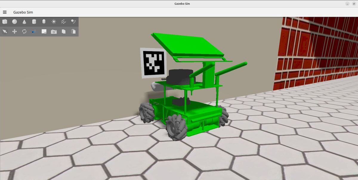
export GZ_SIM_RESOURCE_PATH=/home/ubuntu/ros2_ws/src/yahboom_rosmaster/yahboom_rosmaster_gazebo/modelsNow launch your Gazebo world:
gz sim cafe.worldYour Gazebo world should now include the April Tag.
Remember to adjust the pose of the AprilTag as needed to ensure it is visible and correctly placed in your specific world layout.
Convert the Raw Camera Images into Rectified Images
Let’s create a launch file that will use the image_proc package’s rectify node to do the following:
Subscribes to:
- /cam_1/color/image_raw (sensor_msgs/msg/Image)
- /cam_1/color/camera_info (sensor_msgs/msg/CameraInfo)
Publishes:
- /cam_1/color/image_rect (sensor_msgs/msg/Image)
Open a terminal window, and type:
cd ~/ros2_ws/src/yahboom_rosmaster/yahboom_rosmaster_docking/mkdir launchAdd this file to the launch folder:
apriltag_dock_pose_publisher.launch.pySave the file, and close it.
Edit CMakeLists.txt.
Add these lines:
# Copy necessary files to designated locations in the project
install (
  DIRECTORY launch
  DESTINATION share/${PROJECT_NAME}
)
Save the file, and close it.
Build your workspace.
cd ~/ros2_ws/colcon build && source ~/.bashrcLaunch the robot.
navOnce everything is up, type:
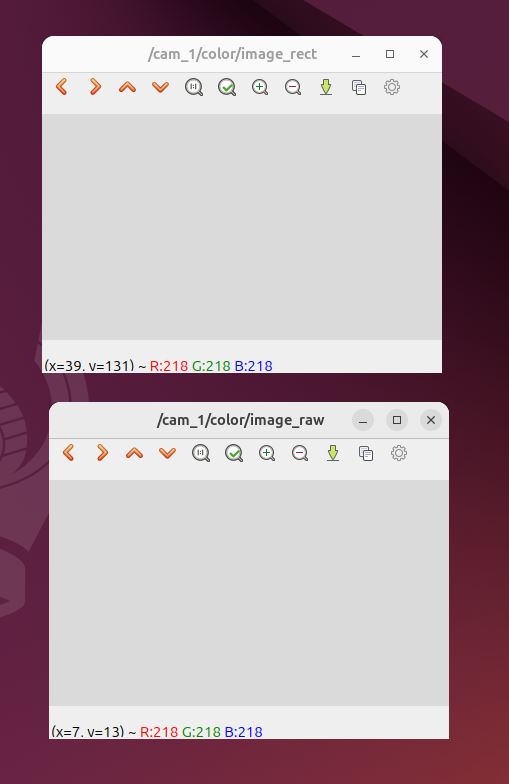
ros2 launch yahboom_rosmaster_docking apriltag_dock_pose_publisher.launch.pyTo see the rectified image:
ros2 run image_view image_view --ros-args -r image:=/cam_1/color/image_rectRun the image viewer to see the raw input image:
ros2 run image_view image_view --ros-args -r image:=cam_1/color/image_rawYou should see a light grey square in both images.
Type this command in the terminal window:
ros2 topic list | grep cam_1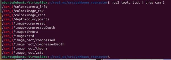
You can safely ignore the synchronization warnings. These warnings happen from time to time due to minor timing misalignments with Gazebo.
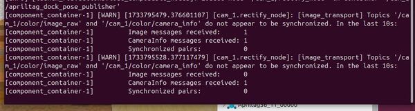
The important thing is that you can see the rectified image properly. Feel free to move the robot around.
Publish the April Tag Pose Using the apriltag_ros Package
We will now use the apriltag_ros package to publish the pose of the AprilTag with respect to the camera’s optical frame.
Specifically, we will detect our tag (ID 0 from family 36h11) in the rectified camera image and then publish the following coordinate transformation:
- Parent frame: cam_1_depth_optical_frame (our camera’s optical frame)
- Child frame: tag36h11:0 (our AprilTag’s frame)
Let’s start by creating a configuration file.
Open a terminal window, and type:
cd ~/ros2_ws/src/yahboom_rosmaster/yahboom_rosmaster_docking/mkdir configAdd this file to the config folder:
apriltags_36h11.yamlSave the file, and close it.
Edit CMakeLists.txt.
Add these lines:
# Copy necessary files to designated locations in the project
install (
  DIRECTORY config launch
  DESTINATION share/${PROJECT_NAME}
)
Save the file, and close it.
Build your workspace.
cd ~/ros2_ws/colcon build && source ~/.bashrcLet’s test our AprilTag detection pipeline. First, make sure your robot is running:
navOnce your robot is up and running, open a new terminal and launch our AprilTag detection nodes:
ros2 launch yahboom_rosmaster_docking apriltag_dock_pose_publisher.launch.pyNavigate your robot to where it can see the AprilTag in its front camera.
Now let’s verify that our AprilTag detection pipeline is working correctly. Open a new terminal and check if we’re receiving AprilTag detections:
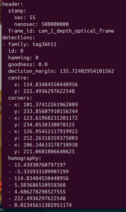
ros2 topic echo /cam_1/detectionsYou should see detection messages whenever your robot’s camera sees the AprilTag. These messages include information about the tag’s ID, position, and detection confidence.
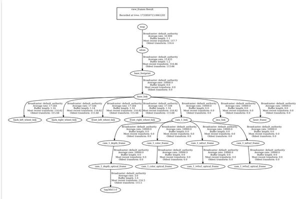
To verify the coordinate transformations are being published correctly, use the tf2_tools package:
ros2 run tf2_tools view_framesThis command will generate a PDF file showing the complete transform tree. Look for a transform from cam_1_depth_optical_frame to tag36h11:0.
To see these transforms in real-time, open another terminal and type:
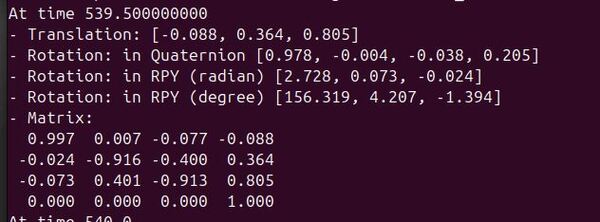
ros2 run tf2_ros tf2_echo cam_1_depth_optical_frame tag36h11:0This will display the position and orientation of the tag relative to your robot’s camera optical frame, updating in real-time.
You can also visualize what your robot’s camera is seeing. To view the rectified image (which is what the AprilTag detector uses):
ros2 run image_view image_view --ros-args -r image:=/cam_1/color/image_rect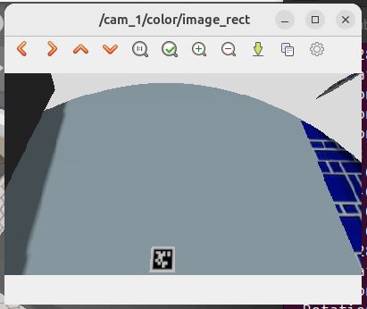
Try moving your robot around to different positions where it can see the AprilTag. You should observe:
- The detection messages updating in the topic echo window
- The transform values changing as the relative position between camera and tag changes
- The AprilTag visible in the image viewer windows
Let me explain the transform from the camera’s optical frame to the AprilTag frame. Remember that we’re working with rectified images, which means the image has been processed to remove lens distortion and appear as if taken by an ideal camera.
In the camera’s optical frame (assume we are in front of the camera looking directly at the camera lens):
- Positive X points to the left
- Positive Y points down
- Positive Z points outward from the camera lens towards us
For the AprilTag (assume we are looking directly at the tag above the docking station, which is against the wall):
- Positive Z points out from the tag towards us (away from the wall and into the scene)
- Positive X points to the right of the tag
- Positive Y points up along the tag towards the ceiling
The translation [-0.088, 0.364, 0.805] tells us the tag’s position relative to the camera optical frame (assume we are looking through the camera lens at the AprilTag):
- -0.088m in X: Tag is slightly to the left of the camera’s center
- +0.364m in Y: Tag appears in the lower portion of the image
- +0.805m in Z: Tag is about 0.8 meters in front of the camera
The rotation, shown in degrees [156.319, 4.207, -1.394], represents:
- Roll (156.319°): This large value indicates the tag is mounted vertically on the wall. The tag orientation is achieved by rotating the camera optical frame (parent) about its x axis 156 degrees in the counterclockwise direction so that it aligns with the child tag36h11:0 frame (remember the right-hand rule of robotics)
- Pitch (4.207°): Small positive pitch shows the tag is almost directly facing the camera
- Yaw (-1.394°): Minimal yaw means the tag is mounted level on the wall with almost no rotation to the left or right
The transform matrix combines both the rotation and translation into a single 4×4 matrix, useful for computing the exact pose of the tag relative to the camera. This information will be essential for our docking system to determine how to approach the dock.
If you’re seeing the AprilTag detections and transforms being published, congratulations! Your AprilTag detection pipeline is working correctly.
I will now add the apriltag_dock_pose_publisher.launch.py launch file to the main navigation launch file rosmaster_x3_navigation.launch.py, which is inside the yahboom_rosmaster_bringup/launch folder.
Create a Detected Dock Pose Publisher
To make our docking system work with AprilTags, we need to create a node that will listen to the /tf topic for the transform between the cam_1_depth_optical_frame (parent frame) and the tag36h11:0 child frame. It will then publish this information as a geometry_msgs/PoseStamped message to a topic named detected_dock_pose.
Our Detected Dock Pose Publisher will process this transformation information and publish the dock’s AprilTag pose as a geometry_msgs/PoseStamped message on the “detected_dock_pose” topic. This publisher is important because it transforms the AprilTag pose data from the TF tree into a format that the docking system can directly use to locate and approach the dock accurately.
The Nav2 Docking Server uses the information on the detected_dock_pose topic through its SimpleChargingDock plugin. Looking at the SimpleChargingDock source code, this plugin specifically subscribes to:
- detected_dock_pose (geometry_msgs/msg/PoseStamped) – For getting the current pose of the AprilTag associated with the docking station
Let’s to create a node to add to our yahboom_rosmaster_navigation package that:
- Listens for the cam_1_depth_optical_frame to tag36h11:0 transform.
- Publishes this as a PoseStamped message to the detected_dock_pose topic with the “cam_1_depth_optical_frame” frame as the default frame_id in the header. The reference code here from NVIDIA serves as a rough guide to what we must do.
Open a terminal window, and type:
cd ~/ros2_ws/src/yahboom_rosmaster/yahboom_rosmaster_docking/srctouch detected_dock_pose_publisher.cppAdd this code.
Save the file, and close it.
Update your CMakeLists.txt.
Now add this node to your apriltag_dock_pose_publisher.launch.py launch file in the yahboom_rosmaster_docking package.
Also uncomment the relevant lines in your main launch file: rosmaster_x3_navigation.launch.py.
Build the package.
cd ~/ros2_ws/ && colcon build && source ~/.bashrcTo test that everything is setup properly, launch the robot:
navNow run the following command:
ros2 topic info /detected_dock_pose -vYou should see one publisher (detected_dock_pose_publisher) and one subscriber (docking_server).
Navigate the robot over to the AprilTag so that the tag is in the camera’s field of view. Then type:
ros2 topic echo /detected_dock_pose My output is this:
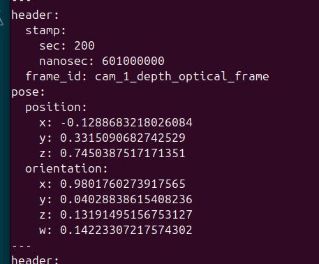
The data should match the output from this command:
ros2 run tf2_ros tf2_echo cam_1_depth_optical_frame tag36h11:0To see what the camera sees, type:
ros2 run image_view image_view --ros-args -r image:=/cam_1/color/image_rectOverview of the Docking Action
Now that we have the data setup, it is time to configure the docking server for Nav2.
The docking action in Nav2 guides your robot from its current position to a successful connection with a charging dock. Here’s a high-level overview of how it works:
- The action server receives a request to dock, either specifying a dock ID from a known database or providing explicit dock pose information.
- If the robot isn’t already near the dock, it uses Nav2 to navigate to a predefined staging pose near the charging station.
- Once at the staging pose, the robot begins to search for and detect the April tag associated with the dock.
- Using visual feedback from the AprilTag, the robot enters a precision control loop, carefully maneuvering to align itself with the dock.
- The robot continues its approach until it detects contact with the dock or confirms that charging has begun.
- If the docking attempt fails, the system can retry the process a configurable number of times.
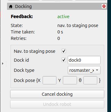
- Throughout the process, the action server provides feedback on the current state and elapsed time.
This structured approach allows for reliable docking across various robot types and environments, with the flexibility to handle different dock designs and detection methods.
Overview of the Undocking Action
The undocking action in Nav2 guides your robot from a docked position to a safe staging pose away from the charging station. Here’s a high-level overview of how it works:
- The action server receives a request to undock, optionally including the dock type if not already known from a previous docking operation.
- The system verifies the dock type and current docking status, ensuring the robot is actually docked (for charging docks).
- For charging docks, the system first attempts to disable charging before any physical movement begins.
- Once charging is disabled, the robot calculates its staging pose based on its current position relative to the dock.
- Using a precision control loop, the robot carefully maneuvers to the staging pose while maintaining specified linear and angular tolerances.
- The system monitors both position and charging status, only considering the undocking successful when the robot has reached the staging pose and charging has completely stopped.
- Throughout the process, the system enforces timeout limits and can respond to cancellation requests for safety.
This structured approach allows for reliable undocking that works across different robot platforms and dock types, while maintaining the safety and integrity of both the robot and charging equipment.
Create the Dock Database File
To use the Nav2 docking server, you’ll need to create a database of known docking stations in your environment. This database tells your robot where docks are located and what type they are. Here’s how to set it up. We will store our files in the yahboom_rosmaster_docking package.
You can find a guide of how to create the database file here on GitHub.
Open a terminal window, and type:
cd ~/ros2_ws/src/yahboom_rosmaster/yahboom_rosmaster_docking/configtouch dock_database.yaml Add this code.
Save the file, and close it.
In this file, we defined a dock with a unique identifier, its type, and its pose in your map. The pose is given as [x, y, theta] coordinates.
Configure the Docking Server
We now need to configure the docking_server.
First, let’s navigate to the folder where the Nav2 parameters are located.
Open a terminal and move to the config folder.
cd ~/ros2_ws/src/yahboom_rosmaster/yahboom_rosmaster_navigation/config/Now, let’s open the YAML file using a text editor: rosmaster_x3_nav2_default_params.yaml
Add these parameters.
docking_server:
  ros__parameters:
    controller_frequency: 10.0
    initial_perception_timeout: 20.0  # Default 5.0
    wait_charge_timeout: 5.0
    dock_approach_timeout: 30.0
    undock_linear_tolerance: 0.05
    undock_angular_tolerance: 0.05
    max_retries: 3
    base_frame: "base_link"
    fixed_frame: "odom"
    dock_backwards: false
    dock_prestaging_tolerance: 0.5

    # Types of docks
    dock_plugins: ['rosmaster_x3_dock']
    rosmaster_x3_dock:
      plugin: 'opennav_docking::SimpleChargingDock'
      docking_threshold: 0.02
      staging_x_offset: 0.75
      staging_yaw_offset: 3.14
      use_external_detection_pose: true
      use_battery_status: false
      use_stall_detection: false
      stall_velocity_threshold: 1.0
      stall_effort_threshold: 1.0
      charging_threshold: 0.5

      external_detection_timeout: 1.0
      external_detection_translation_x: -0.18
      external_detection_translation_y: 0.0
      external_detection_rotation_roll: -1.57
      external_detection_rotation_pitch: 1.57
      external_detection_rotation_yaw: 0.0
      filter_coef: 0.1

    # Dock instances
    dock_database: $(find-pkg-share yahboom_rosmaster_docking)/config/dock_database.yaml

    controller:
      k_phi: 3.0
      k_delta: 2.0
      beta: 0.4
      lambda: 2.0
      v_linear_min: 0.1
      v_linear_max: 0.15
      v_angular_max: 0.75
      slowdown_radius: 0.25
      use_collision_detection: true
      costmap_topic: "/local_costmap/costmap_raw"
      footprint_topic: "/local_costmap/published_footprint"
      transform_tolerance: 0.1
      projection_time: 5.0
      simulation_step: 0.1
      dock_collision_threshold: 0.3
Save the file, and close it.
You can find a detailed list and description of each of these parameters here.
In this scenario, the docking camera is on the front of the robot. Remember ROS conventions:
For the AprilTag (assume we are looking directly at the tag on the docking station):
- Z-axis points out from the tag (away from the docking station, towards us)
- X-axis points to the right of the tag
- Y-axis points up along the tag towards the celing
For the robot’s base_link:
- X-axis points forward
- Y-axis points left
- Z-axis points up
The docking pose of the robot is the AprilTag’s pose with certain translations and rotations applied.
The external_detection_* values in the docking parameters define offsets relative to the AprilTag frame to specify where the robot should dock.
We use the right hand rule here to figure out the values for the external_detection translations and rotations.
To properly express the docking pose relative to the AprilTag’s pose, we need to figure out what combination of rotations and translations of the parent AprilTag axes will match up to the desired docking pose.
You can see in the source code that the rotations are applied in this order: pitch (rotation around the y-axis by 90 degrees counterclockwise…1.57 radians), roll (rotation around the x-axis 90 degrees clockwise…-1.57 radians), then yaw (no rotation around the z-axis).
When you use your right hand to perform these rotations, you will see that your hand will align with the expected orientation of the robot when it is parked headfirst into the docking station.
Since the x-axis of the AprilTag points to the right (as if we are looking directly at the tag), we need that axis to point forward so that it is aligned with the robot base link forward direction x-axis.
To do this, we first rotate the AprilTag pose around its y axis (our middle finger). The z-x plane rotates counterclockwise around the positive y-axis 90 degrees. Counterclockwise rotations in robotics are positive by convention, so we have 1.5708 for external_detection_rotation_pitch. Remember pitch is another way of saying rotation around the y-axis.
Now we need to get the z-axis of the AprilTag pointing towards the sky. To do that, we need to rotate clockwise around the positive x-axis 90 degrees (imagine we are looking down at the arrow of the positive x-axis and watching the y-z plane rotate…rotate around your index finger). Clockwise rotations in robotics are negative by convention, so we have -1.5708 for external_detection_rotation_roll. Remember roll is another way of saying rotation around the x-axis.
Now our AprilTag orientation is aligned with the axes of the robot. Your thumb should be pointing towards the ceiling.
We then move 0.18 meters down the negative x-axis (move your forearm backwards in the direction of your elbow) to get to the desired docking position of the robot. That is why external_detection_translation_x = -0.18.
In robotics and computer graphics, translations and rotations are generally non-commutative – meaning the order in which you apply them produces different results. Remember you need to:
- First correct the orientation of the parent frame to match your expected child frame orientation.
- Then apply any translational offsets based on that corrected orientation
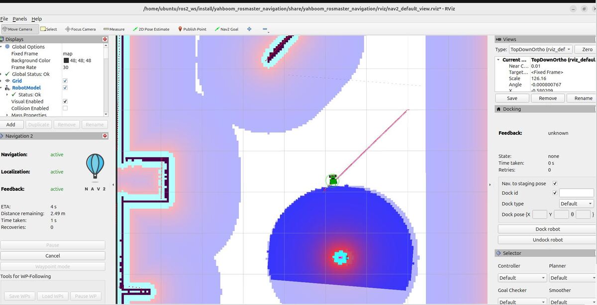
Test Docking and Undocking
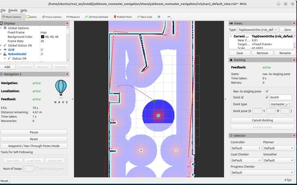
Now let’s send the robot to the dock using RViz.
Build your workspace.
cd ~/ros2_ws/colcon build && source ~/.bashrcLaunch navigation.
navOnce everything has come up, go to the right panel.
In the Dock id field, type dock0. This is the id of the docking station.
Next to Dock type, select rosmaster_x3_dock.
Click Dock robot.
We could have also done this:
ros2 action send_goal /dock_robot nav2_msgs/action/DockRobot "{use_dock_id: true, dock_id: 'dock0', dock_type: 'rosmaster_x3_dock', max_staging_time: 1000.0, navigate_to_staging_pose: true}"
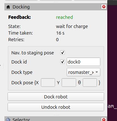
To undock the robot, either click the Undock robot button in RViz, or type:
ros2 action send_goal /undock_robot nav2_msgs/action/UndockRobot "{dock_type: 'rosmaster_x3_dock', max_undocking_time: 30.0}"The nav2_docking server doesn’t allow a lot of control over the undocking process. I would prefer to just back out straight to the staging pose. I had best results by shortening the max_undocking_time to 2.0 seconds, letting the action abort, and then sending a regular navigation goal after that. This package is fairly new as of the time of this writing, and definitely needs a little more work to be ready for prime time.
ros2 action send_goal /undock_robot nav2_msgs/action/UndockRobot "{dock_type: 'rosmaster_x3_dock', max_undocking_time: 2.0}"That’s it.
If you want to take the work we did here to the next level, you can send docking and undocking goals by creating action clients that connect to the /dock_robot and /undock_robot action servers. You can write these clients using the Simple Commander API if you want to use Python, or you can use C++.
Keep building!
Getting Started With the Simple Commander API – ROS 2 Jazzy
In this tutorial, we will explore the Nav2 Simple Commander API, a powerful tool that simplifies robot navigation programming in Python. We’ll learn how to use this API to control a robot’s movement, plan paths, and execute various navigation tasks without getting bogged down in complex ROS 2 details. This guide will help you get started with the most important features of the Simple Commander API.
By the end of this tutorial, you will be able to build this:
Real-World Applications
You can use the Nav2 Simple Commander API in many real-world situations. Here are some examples:
- Home Help: You can create robots that clean your house or bring you things from other rooms.
- Warehouse Work: You can build robots that check items on shelves or pick up and move things around the warehouse.
- Farming: You can develop vehicles that plant, check, or pick crops.
- Security: You can make robots that patrol areas or quickly go to places where there might be trouble.
- Healthcare: You can create robots that bring medicine to hospital rooms or clean areas to keep them safe.
Prerequisites
- You have completed this tutorial: Autonomous Navigation for a Mobile Robot Using ROS 2 Jazzy.
All my code for this project is located here on GitHub.
Create Folders
To get started with the Nav2 Simple Commander API, you’ll need to set up your workspace. Follow these steps to create the necessary folders:
Open a terminal window, and type the following command:
cd ~/ros2_ws/src/yahboom_rosmaster/yahboom_rosmaster_navigationCreate a folder for your Python scripts:
mkdir scriptsCreate a folder for the helper files you will create:
mkdir yahboom_rosmaster_navigationcd yahboom_rosmaster_navigationtouch __init__.pyCreate a Goal Pose Message Generator
Now we will create a goal pose message generator. This generator is important for our navigation tasks because:
- In ROS 2, robot positions and orientations are often represented using the PoseStamped message type.
- This message type includes not just the position and orientation, but also timing and reference frame information, which are essential for accurate navigation.
- Creating a function to generate these messages will simplify our code when we need to specify goal positions for our robot.
Open a terminal window:
cd ~/ros2_ws/src/yahboom_rosmaster/yahboom_rosmaster_navigation/yahboom_rosmaster_navigation/touch posestamped_msg_generator.pyType this code.
#!/usr/bin/env python3
"""
Create a PoseStamped message for ROS 2 navigation.

This script creates a geometry_msgs/PoseStamped message which is commonly used
for robot navigation in ROS 2. It shows how to properly construct a PoseStamped
message with header information and pose data.

:author: Addison Sears-Collins
:date: December 5, 2024
"""

from rclpy.node import Node
from builtin_interfaces.msg import Time
from geometry_msgs.msg import PoseStamped, Pose, Point, Quaternion
from std_msgs.msg import Header


class PoseStampedGenerator(Node):
    """A ROS 2 node that generates PoseStamped messages."""

    def __init__(self, node_name='pose_stamped_generator'):
        """
        Initialize the ROS 2 node.

        :param node_name: Name of the node
        :type node_name: str
        """
        super().__init__(node_name)

    def create_pose_stamped(self, x=0.0, y=0.0, z=0.0,
                            qx=0.0, qy=0.0, qz=0.0, qw=1.0,
                            frame_id='map'):
        """
        Create a PoseStamped message with the specified parameters.

        :param x: x position coordinate
        :type x: float
        :param y: y position coordinate
        :type y: float
        :param z: z position coordinate
        :type z: float
        :param qx: x quaternion component
        :type qx: float
        :param qy: y quaternion component
        :type qy: float
        :param qz: z quaternion component
        :type qz: float
        :param qw: w quaternion component
        :type qw: float
        :param frame_id: reference frame
        :type frame_id: str
        :return: pose stamped message
        :rtype: PoseStamped
        """
        # Create the PoseStamped message object
        pose_stamped = PoseStamped()

        # Create and fill the header with frame_id and timestamp
        header = Header()
        header.frame_id = frame_id

        # Get current ROS time and convert to Time message
        now = self.get_clock().now()
        header.stamp = Time(
            sec=now.seconds_nanoseconds()[0],
            nanosec=now.seconds_nanoseconds()[1]
        )

        # Create and fill the position message with x, y, z coordinates
        position = Point()
        position.x = float(x)
        position.y = float(y)
        position.z = float(z)

        # Create and fill the orientation message with quaternion values
        orientation = Quaternion()
        orientation.x = float(qx)
        orientation.y = float(qy)
        orientation.z = float(qz)
        orientation.w = float(qw)

        # Create Pose message and combine position and orientation
        pose = Pose()
        pose.position = position
        pose.orientation = orientation

        # Combine header and pose into the final PoseStamped message
        pose_stamped.header = header
        pose_stamped.pose = pose

        return pose_stamped
Save the file, and close it.
This script provides a ROS 2 node class PoseStampedGenerator that creates geometry_msgs/PoseStamped messages. The class provides a create_pose_stamped method that takes:
- Position coordinates (x, y, z)
- Orientation as a quaternion (qx, qy, qz, qw)
- Reference frame (defaults to ‘map’)
Create a Go to Goal Pose Script
Now I will show you how to create a script that will send a robot to a single goal location (i.e. “goal pose”). A barebones official example code for sending a single goal is here on the Nav2 GitHub. However, this code is missing some important functionality that you will need for a real-world production mobile robot that needs to navigate in a dynamic environment with people moving around and objects of all shapes and sizes. For this reason, we are going to use that code as a basis and then add additional functionality.
Our navigation script will assume the initial pose of the robot has already been set either via RViz, the command line, or some other method.
To create this script, open a terminal, and navigate to the scripts directory:
cd ~/ros2_ws/src/yahboom_rosmaster_navigation/yahboom_rosmaster_navigation/scriptstouch nav_to_pose.pyAdd this code.
#!/usr/bin/env python3
"""
ROS 2 node for navigating to a goal pose and publishing status updates.

This script creates a ROS 2 node that:
    - Subscribes to a goal pose
    - Navigates the robot to the goal pose
    - Publishes the estimated time of arrival
    - Publishes the goal status
    - Cancels the goal if a stop signal is received

Subscription Topics:
    /goal_pose/goal (geometry_msgs/PoseStamped): The desired goal pose
    /stop/navigation/go_to_goal_pose (std_msgs/Bool): Signal to stop navigation
    /cmd_vel (geometry_msgs/Twist): Velocity command

Publishing Topics:
    /goal_pose/eta (std_msgs/String): Estimated time of arrival in seconds
    /goal_pose/status (std_msgs/String): Goal pose status

:author: Addison Sears-Collins
:date: December 5, 2024
"""

import time
import rclpy
from rclpy.duration import Duration
from rclpy.executors import MultiThreadedExecutor
from rclpy.node import Node
from nav2_simple_commander.robot_navigator import BasicNavigator, TaskResult
from std_msgs.msg import Bool, String
from geometry_msgs.msg import Twist, PoseStamped

# Global flags for navigation state
STOP_NAVIGATION_NOW = False
NAV_IN_PROGRESS = False
MOVING_FORWARD = True

COSTMAP_CLEARING_PERIOD = 0.5


class GoToGoalPose(Node):
    """This class subscribes to the goal pose and publishes the ETA
       and goal status information to ROS 2.
    """

    def __init__(self):
        """Constructor."""
        # Initialize the class using the constructor
        super().__init__('go_to_goal_pose')

        # Create the ROS 2 publishers
        self.publisher_eta = self.create_publisher(String, '/goal_pose/eta', 10)
        self.publisher_status = self.create_publisher(String, '/goal_pose/status', 10)

        # Create a subscriber
        # This node subscribes to messages of type geometry_msgs/PoseStamped
        self.subscription_go_to_goal_pose = self.create_subscription(
            PoseStamped,
            '/goal_pose/goal',
            self.go_to_goal_pose,
            10)

        # Keep track of time for clearing the costmaps
        self.current_time = self.get_clock().now().nanoseconds
        self.last_time = self.current_time
        self.dt = (self.current_time - self.last_time) * 1e-9

        # Clear the costmap every X.X seconds when the robot is not making forward progress
        self.costmap_clearing_period = COSTMAP_CLEARING_PERIOD

        # Launch the ROS 2 Navigation Stack
        self.navigator = BasicNavigator()

        # Wait for navigation to fully activate
        self.navigator.waitUntilNav2Active()

    def go_to_goal_pose(self, msg):
        """Go to goal pose."""
        global NAV_IN_PROGRESS, STOP_NAVIGATION_NOW  # pylint: disable=global-statement

        # Clear all costmaps before sending to a goal
        self.navigator.clearAllCostmaps()

        # Go to the goal pose
        self.navigator.goToPose(msg)

        # As long as the robot is moving to the goal pose
        while rclpy.ok() and not self.navigator.isTaskComplete():
            # Get the feedback message
            feedback = self.navigator.getFeedback()

            if feedback:
                # Publish the estimated time of arrival in seconds
                estimated_time_of_arrival = f"{Duration.from_msg(
                    feedback.estimated_time_remaining).nanoseconds / 1e9:.0f}"
                msg_eta = String()
                msg_eta.data = str(estimated_time_of_arrival)
                self.publisher_eta.publish(msg_eta)

                # Publish the goal status
                msg_status = String()
                msg_status.data = "IN_PROGRESS"
                self.publisher_status.publish(msg_status)
                NAV_IN_PROGRESS = True

                # Clear the costmap at the desired frequency
                # Get the current time
                self.current_time = self.get_clock().now().nanoseconds

                # How much time has passed in seconds since the last costmap clearing
                self.dt = (self.current_time - self.last_time) * 1e-9

                # If we are making no forward progress after X seconds, clear all costmaps
                if not MOVING_FORWARD and self.dt > self.costmap_clearing_period:
                    self.navigator.clearAllCostmaps()
                    self.last_time = self.current_time

            # Stop the robot if necessary
            if STOP_NAVIGATION_NOW:
                self.navigator.cancelTask()
                self.get_logger().info('Navigation cancellation request fulfilled...')

            time.sleep(0.1)

        # Reset the variable values
        STOP_NAVIGATION_NOW = False
        NAV_IN_PROGRESS = False

        # Publish the final goal status
        result = self.navigator.getResult()
        msg_status = String()

        if result == TaskResult.SUCCEEDED:
            self.get_logger().info('Successfully reached the goal!')
            msg_status.data = "SUCCEEDED"
            self.publisher_status.publish(msg_status)

        elif result == TaskResult.CANCELED:
            self.get_logger().info('Goal was canceled!')
            msg_status.data = "CANCELED"
            self.publisher_status.publish(msg_status)

        elif result == TaskResult.FAILED:
            self.get_logger().info('Goal failed!')
            msg_status.data = "FAILED"
            self.publisher_status.publish(msg_status)

        else:
            self.get_logger().info('Goal has an invalid return status!')
            msg_status.data = "INVALID"
            self.publisher_status.publish(msg_status)


class GetStopNavigationSignal(Node):
    """This class subscribes to a Boolean flag that tells the
       robot to stop navigation.
    """

    def __init__(self):
        """Constructor."""
        # Initialize the class using the constructor
        super().__init__('get_stop_navigation_signal')

        # Create a subscriber
        # This node subscribes to messages of type std_msgs/Bool
        self.subscription_stop_navigation = self.create_subscription(
            Bool,
            '/stop/navigation/go_to_goal_pose',
            self.set_stop_navigation,
            10)

    def set_stop_navigation(self, msg):
        """Determine if the robot needs to stop, and adjust the variable value accordingly."""
        global STOP_NAVIGATION_NOW  # pylint: disable=global-statement

        if NAV_IN_PROGRESS and msg.data:
            STOP_NAVIGATION_NOW = msg.data
            self.get_logger().info('Navigation cancellation request received by ROS 2...')


class GetCurrentVelocity(Node):
    """This class subscribes to the current velocity and determines if the robot
       is making forward progress.
    """

    def __init__(self):
        """Constructor."""
        # Initialize the class using the constructor
        super().__init__('get_current_velocity')

        # Create a subscriber
        # This node subscribes to messages of type geometry_msgs/Twist
        self.subscription_current_velocity = self.create_subscription(
            Twist,
            '/cmd_vel',
            self.get_current_velocity,
            1)

    def get_current_velocity(self, msg):
        """Get the current velocity, and determine if the robot is making forward progress."""
        global MOVING_FORWARD  # pylint: disable=global-statement

        linear_x_value = msg.linear.x

        if linear_x_value <= 0.0:
            MOVING_FORWARD = False
        else:
            MOVING_FORWARD = True


def main(args=None):
    """Main function to initialize and run the ROS 2 nodes."""
    # Initialize the rclpy library
    rclpy.init(args=args)

    try:
        # Create the nodes
        go_to_goal_pose = GoToGoalPose()
        get_stop_navigation_signal = GetStopNavigationSignal()
        get_current_velocity = GetCurrentVelocity()

        # Set up multithreading
        executor = MultiThreadedExecutor()
        executor.add_node(go_to_goal_pose)
        executor.add_node(get_stop_navigation_signal)
        executor.add_node(get_current_velocity)

        try:
            # Spin the nodes to execute the callbacks
            executor.spin()
        finally:
            # Shutdown the nodes
            executor.shutdown()
            go_to_goal_pose.destroy_node()
            get_stop_navigation_signal.destroy_node()
            get_current_velocity.destroy_node()

    finally:
        # Shutdown the ROS client library for Python
        rclpy.shutdown()


if __name__ == '__main__':
    main()
Save the code, and close it.
Our navigation script, nav_to_pose.py, works as follows:
It sets up three ROS 2 nodes.
The GoToGoalPose node:
- Subscribes to goal poses and initiates navigation.
- Publishes estimated time of arrival (ETA) and navigation status.
- Handles navigation feedback and result processing.
- Implements costmap clearing to handle dynamic obstacles.
The GetStopNavigationSignal node allows external cancellation of navigation tasks.
The GetCurrentVelocity node monitors if the robot is moving forward, which is used for costmap clearing decisions.
The script uses a multithreaded executor to run all nodes concurrently.
It implements error handling and proper shutdown procedures.
Key features include:
- Dynamic obstacle handling through costmap clearing.
- Real-time status and ETA updates.
- Ability to cancel navigation tasks.
- Robust error handling and graceful shutdown.
Once we area ready to test the navigation, we will send a goal pose from the command line:
ros2 topic pub /goal_pose/goal geometry_msgs/PoseStamped "{header: {stamp: {sec: 0, nanosec: 0}, frame_id: 'map'}, pose: {position: {x: 2.0, y: 2.0, z: 0.0}, orientation: {x: 0.0, y: 0.0, z: 0.7071068, w: 0.7071068}}}" --onceAlternatively, we can use a script to send the goal. Let’s create a script called test_nav_to_pose.py:
In the same directory, create and open the file:
touch test_nav_to_pose.pyAdd this code.
#!/usr/bin/env python3
"""
ROS 2 node for sending a robot to different tables based on user input.

This script creates a ROS 2 node that continuously prompts the user to select a table
number (1-5) in the cafe world and publishes the corresponding goal pose for the
robot to navigate to. The script will keep running until the user enters 'q' or presses Ctrl+C.

Publishing Topics:
    /goal_pose/goal (geometry_msgs/PoseStamped): The desired goal pose for the robot

:author: Addison Sears-Collins
:date: December 5, 2024
"""

import rclpy
from rclpy.node import Node
from geometry_msgs.msg import PoseStamped
from yahboom_rosmaster_navigation.posestamped_msg_generator import PoseStampedGenerator


class GoalPublisher(Node):
    """
    ROS 2 node for publishing goal poses to different tables.

    This node allows users to input table numbers and publishes the corresponding
    goal poses for robot navigation.

    Attributes:
        publisher: Publisher object for goal poses
        locations (dict): Dictionary containing x,y coordinates for each table
        pose_generator: Generator for PoseStamped messages
    """

    def __init__(self):
        """
        Initialize the GoalPublisher node.

        Sets up the publisher for goal poses and defines the table locations.
        """
        super().__init__('goal_publisher')

        # Create a publisher that will send goal poses to the robot
        self.publisher = self.create_publisher(PoseStamped, '/goal_pose/goal', 10)
        self.get_logger().info('Goal Publisher node has been initialized')

        # Initialize the PoseStamped message generator
        self.pose_generator = PoseStampedGenerator('pose_generator')

        # Dictionary storing the x,y coordinates for each table
        self.locations = {
            '1': {'x': -0.96, 'y': -0.92},   # Table 1 location
            '2': {'x': 1.16, 'y': -4.23},    # Table 2 location
            '3': {'x': 0.792, 'y': -8.27},   # Table 3 location
            '4': {'x': -3.12, 'y': -7.495},  # Table 4 location
            '5': {'x': -2.45, 'y': -3.55}    # Table 5 location
        }

    def publish_goal(self, table_number):
        """
        Publish a goal pose for the selected table.

        Creates and publishes a PoseStamped message with the coordinates
        corresponding to the selected table number.

        Args:
            table_number (str): The selected table number ('1' through '5')
        """
        # Get the coordinates for the selected table
        x = self.locations[table_number]['x']
        y = self.locations[table_number]['y']

        # Create the PoseStamped message using the generator
        # Using default orientation (facing forward) and z=0.0
        pose_msg = self.pose_generator.create_pose_stamped(
            x=x,
            y=y,
            z=0.0,
            qx=0.0,
            qy=0.0,
            qz=0.0,
            qw=1.0,
            frame_id='map'
        )

        # Publish the goal pose
        self.publisher.publish(pose_msg)
        self.get_logger().info(f'Goal pose published for table {table_number}')

    def run_interface(self):
        """
        Run the user interface for table selection.

        Continuously prompts the user to select a table number and publishes
        the corresponding goal pose. Exits when user enters 'q' or Ctrl+C.
        """
        while True:
            # Display available tables
            print("\nAVAILABLE TABLES:")
            for table in self.locations:
                print(f"Table {table}")

            # Get user input
            user_input = input('\nEnter table number (1-5) or "q" to quit: ').strip()

            # Check if user wants to quit
            if user_input.lower() == 'q':
                break

            # Validate and process user input
            if user_input in self.locations:
                self.publish_goal(user_input)
            else:
                print("Invalid table number! Please enter a number between 1 and 5.")


def main(args=None):
    """
    Main function to initialize and run the ROS 2 node.

    Args:
        args: Command-line arguments (default: None)
    """
    # Initialize ROS 2
    rclpy.init(args=args)

    # Create and run the node
    goal_publisher = GoalPublisher()

    try:
        goal_publisher.run_interface()
    except KeyboardInterrupt:
        print("\nShutting down...")
    finally:
        # Clean up
        goal_publisher.destroy_node()
        rclpy.shutdown()


if __name__ == '__main__':
    main()
Save the code, and close it.
This Python script creates a ROS 2 node that lets you send a robot to different predefined table locations in a cafe environment by entering table numbers (1-5) through a command-line interface. When you select a table number, the code generates and publishes a PoseStamped message containing the x,y coordinates for that table location, which tells the robot where to go. The program runs in a continuous loop asking for your table selections until you quit by entering ‘q’ or pressing Ctrl+C, allowing you to send the robot to multiple locations in sequence.
How to Determine Coordinates for Goals
To determine coordinates for goal locations, open a fresh terminal window, and type:
ros2 topic echo /clicked_pointAt the top of RViz, click the “Publish Point” button.
Click near the first table, and record the coordinates of that point, which will appear in the terminal window.
- table_1: (x=-0.96, y=-0.92)
Now do the same for the other four tables. I will go in a clockwise direction:
- table_2: (x=1.16, y=-4.23)
- table_3: (x=0.792, y=-8.27)
- table_4: (x=-3.12, y=-7.495)
- table_5: (x=-2.45, y=-3.55)
Press CTRL + C when you are done determining the goal locations.
Create an Assisted Teleoperation Script
In this section, we will create an Assisted Teleoperation script for our robot. Assisted Teleoperation allows manual control of the robot while automatically stopping it when obstacles are detected. This feature helps prevent collisions when you are manually sending velocity commands to steer the robot..
You can find a bare-bones example of assisted teleoperation here on the Nav2 GitHub, but we will go beyond that script to make it useful for a real-world environment.
We’ll begin by creating a Python script that implements this functionality:
Open a terminal and navigate to the scripts folder:
cd ~/ros2_ws/src/yahboom_rosmaster/yahboom_rosmaster_navigation/scriptsCreate a new file for assisted teleoperation:
touch assisted_teleoperation.pyAdd the provided code to this file.
#!/usr/bin/env python3
"""
Assisted Teleop Node for ROS 2 Navigation

This script implements an Assisted Teleop node that interfaces with the Nav2 stack.
It manages the lifecycle of the AssistedTeleop action, handles cancellation requests,
and periodically clears costmaps to remove temporary obstacles.

Subscription Topics:
    /cmd_vel_teleop (geometry_msgs/Twist): Velocity commands for assisted teleop
    /cancel_assisted_teleop (std_msgs/Bool): Cancellation requests for assisted teleop

Parameters:
    ~/costmap_clear_frequency (double): Frequency in Hz for costmap clearing. Default: 2.0

:author: Addison Sears-Collins
:date: December 5, 2024
"""

import rclpy
from rclpy.node import Node
from rclpy.exceptions import ROSInterruptException
from geometry_msgs.msg import Twist
from std_msgs.msg import Bool
from nav2_simple_commander.robot_navigator import BasicNavigator
from rcl_interfaces.msg import ParameterDescriptor


class AssistedTeleopNode(Node):
    """
    A ROS 2 node for managing Assisted Teleop functionality.
    """

    def __init__(self):
        """Initialize the AssistedTeleopNode."""
        super().__init__('assisted_teleop_node')

        # Declare and get parameters
        self.declare_parameter(
            'costmap_clear_frequency',
            2.0,
            ParameterDescriptor(description='Frequency in Hz for costmap clearing')
        )
        clear_frequency = self.get_parameter('costmap_clear_frequency').value

        # Initialize the BasicNavigator for interfacing with Nav2
        self.navigator = BasicNavigator('assisted_teleop_navigator')

        # Create subscribers for velocity commands and cancellation requests
        self.cmd_vel_sub = self.create_subscription(
            Twist, '/cmd_vel_teleop', self.cmd_vel_callback, 10)
        self.cancel_sub = self.create_subscription(
            Bool, '/cancel_assisted_teleop', self.cancel_callback, 10)

        # Initialize state variables
        self.assisted_teleop_active = False
        self.cancellation_requested = False

        # Create a timer for periodic costmap clearing with configurable frequency
        period = 1.0 / clear_frequency
        self.clear_costmaps_timer = self.create_timer(period, self.clear_costmaps_callback)

        self.get_logger().info(
            f'Assisted Teleop Node initialized with costmap clearing frequency: {
                clear_frequency} Hz')

        # Wait for navigation to fully activate.
        self.navigator.waitUntilNav2Active()

    def cmd_vel_callback(self, twist_msg: Twist) -> None:
        """Process incoming velocity commands and activate assisted teleop if needed."""
        # Reset cancellation flag when new velocity commands are received
        if (abs(twist_msg.linear.x) > 0.0 or
            abs(twist_msg.linear.y) > 0.0 or
                abs(twist_msg.angular.z) > 0.0):
            self.cancellation_requested = False

        if not self.assisted_teleop_active and not self.cancellation_requested:
            if (abs(twist_msg.linear.x) > 0.0 or
                abs(twist_msg.linear.y) > 0.0 or
                    abs(twist_msg.angular.z) > 0.0):
                self.start_assisted_teleop()

    def start_assisted_teleop(self) -> None:
        """Start the Assisted Teleop action with indefinite duration."""
        self.assisted_teleop_active = True
        self.cancellation_requested = False
        self.navigator.assistedTeleop(time_allowance=0)  # 0 means indefinite duration
        self.get_logger().info('AssistedTeleop activated with indefinite duration')

    def cancel_callback(self, msg: Bool) -> None:
        """Handle cancellation requests for assisted teleop."""
        if msg.data and self.assisted_teleop_active and not self.cancellation_requested:
            self.cancel_assisted_teleop()

    def cancel_assisted_teleop(self) -> None:
        """Cancel the currently running Assisted Teleop action."""
        if self.assisted_teleop_active:
            self.navigator.cancelTask()
            self.assisted_teleop_active = False
            self.cancellation_requested = True
            self.get_logger().info('AssistedTeleop cancelled')

    def clear_costmaps_callback(self) -> None:
        """Periodically clear all costmaps to remove temporary obstacles."""
        if not self.assisted_teleop_active:
            return

        self.navigator.clearAllCostmaps()
        self.get_logger().debug('Costmaps cleared')


def main():
    """Initialize and run the AssistedTeleopNode."""
    rclpy.init()
    node = None

    try:
        node = AssistedTeleopNode()
        rclpy.spin(node)

    except KeyboardInterrupt:
        if node:
            node.get_logger().info('Node shutting down due to keyboard interrupt')
    except ROSInterruptException:
        if node:
            node.get_logger().info('Node shutting down due to ROS interrupt')
    finally:
        if node:
            node.cancel_assisted_teleop()
            node.navigator.lifecycleShutdown()
        rclpy.shutdown()


if __name__ == '__main__':
    main()
This script:
- Subscribes to the /cmd_vel_teleop topic to receive velocity commands from the user.
- Manages the Assisted Teleoperation action in the Nav2 stack.
- Handles cancellation requests for Assisted Teleoperation.
- Periodically clears costmaps to remove temporary obstacles.
- The Nav2 stack processes these commands and publishes the resulting safe velocity commands to the /cmd_vel topic.
It’s important to note that /cmd_vel_teleop is the input topic for user commands, while /cmd_vel is the output topic that sends commands to the robot after processing for obstacle avoidance.
Save and close the file.
Add the Go to Goal Pose and Assisted Teleop Scripts to the Bringup Launch File
Open a terminal window, and type:
cd ~/ros2_ws/src/yahboom_rosmaster/yahboom_rosmaster_bringup/launchOpen rosmaster_x3_navigation.launch.py.
Add our two new nodes:
   start_nav_to_pose_cmd = Node(
        package='yahboom_rosmaster_navigation',
        executable='nav_to_pose.py',
        output='screen',
        parameters=[{'use_sim_time': use_sim_time}]
    )

   start_assisted_teleop_cmd = Node(
        package='yahboom_rosmaster_navigation',
        executable='assisted_teleoperation.py',
        output='screen',
        parameters=[{'use_sim_time': use_sim_time}]
    )

….

   ld.add_action(start_assisted_teleop_cmd)
   ld.add_action(start_nav_to_pose_cmd)
Edit package.xml
To ensure our package has all the necessary dependencies, we need to edit the package.xml file:
Navigate to the package directory:
cd ~/ros2_ws/src/yahboom_rosmaster/yahboom_rosmaster_navigation/Make sure your package.xml looks like this:
<?xml version="1.0"?>
<?xml-model href="http://download.ros.org/schema/package_format3.xsd" schematypens="http://www.w3.org/2001/XMLSchema"?>
<package format="3">
  <name>yahboom_rosmaster_navigation</name>
  <version>0.0.0</version>
  <description>Navigation package for ROSMASTER series robots by Yahboom</description>
  <maintainer email="automaticaddison@todo.com">ubuntu</maintainer>
  <license>BSD-3-Clause</license>

  <buildtool_depend>ament_cmake</buildtool_depend>
  <buildtool_depend>ament_cmake_python</buildtool_depend>

  <depend>rclcpp</depend>
  <depend>rclpy</depend>
  <depend>builtin_interfaces</depend>
  <depend>geometry_msgs</depend>
  <depend>navigation2</depend>
  <depend>nav2_bringup</depend>
  <depend>nav2_simple_commander</depend>
  <depend>slam_toolbox</depend>
  <depend>std_msgs</depend>
  <depend>tf2_ros</depend>
  <depend>tf_transformations</depend>


  <test_depend>ament_lint_auto</test_depend>
  <test_depend>ament_lint_common</test_depend>

  <export>
    <build_type>ament_cmake</build_type>
  </export>
</package>
These dependencies are required for the Assisted Teleoperation functionality to work properly with the Nav2 stack.
Save and close the file.
Edit CMakeLists.txt
To properly build and install all our Python scripts, including the new Assisted Teleoperation script, we need to update the CMakeLists.txt file:
Navigate to the package directory if you’re not already there:
cd ~/ros2_ws/src/yahboom_rosmaster/yahboom_rosmaster_navigation/Open the CMakeLists.txt file:
cmake_minimum_required(VERSION 3.8)
project(yahboom_rosmaster_navigation)

if(CMAKE_COMPILER_IS_GNUCXX OR CMAKE_CXX_COMPILER_ID MATCHES "Clang")
  add_compile_options(-Wall -Wextra -Wpedantic)
endif()

# find dependencies
find_package(ament_cmake REQUIRED)
find_package(ament_cmake_python REQUIRED)
find_package(geometry_msgs REQUIRED)
find_package(navigation2 REQUIRED)
find_package(nav2_bringup REQUIRED)
find_package(rclcpp REQUIRED)
find_package(rclpy REQUIRED)
find_package(slam_toolbox REQUIRED)
find_package(std_msgs REQUIRED)
find_package(tf2_ros REQUIRED)

add_executable(cmd_vel_relay src/cmd_vel_relay_node.cpp)
ament_target_dependencies(cmd_vel_relay
  rclcpp
  geometry_msgs
)

install(TARGETS
  cmd_vel_relay
  DESTINATION lib/${PROJECT_NAME}
)

install (
  DIRECTORY config maps rviz
  DESTINATION share/${PROJECT_NAME}
)

# Install Python modules
ament_python_install_package(${PROJECT_NAME})

# Install Python executables
install(PROGRAMS
  scripts/assisted_teleoperation.py
  scripts/nav_to_pose.py
  scripts/test_nav_to_pose.py
  DESTINATION lib/${PROJECT_NAME}
)

if(BUILD_TESTING)
  find_package(ament_lint_auto REQUIRED)
  # the following line skips the linter which checks for copyrights
  # comment the line when a copyright and license is added to all source files
  set(ament_cmake_copyright_FOUND TRUE)
  # the following line skips cpplint (only works in a git repo)
  # comment the line when this package is in a git repo and when
  # a copyright and license is added to all source files
  set(ament_cmake_cpplint_FOUND TRUE)
  ament_lint_auto_find_test_dependencies()
endif()

ament_package()
Make sure it looks like this.
These changes to CMakeLists.txt will ensure that all our scripts, including the new Assisted Teleoperation script, are properly included when building and installing the package.
Build the Package
Now that we’ve created our scripts and updated the necessary configuration files, it’s time to build our package to incorporate all these changes. This process compiles our code and makes it ready for use in the ROS 2 environment.
Open a terminal window, and type:
cd ~/ros2_wsrosdep install --from-paths src --ignore-src -y -rcolcon build source ~/.bashrcLaunch the Robot
Open a new terminal window, and type the following command to launch the robot. Wait until Gazebo and RViz come fully up, which can take up to 30 seconds:
navor
bash ~/ros2_ws/src/yahboom_rosmaster/yahboom_rosmaster_bringup/scripts/rosmaster_x3_navigation.sh Run Each Script
Let’s test each of the navigation scripts we’ve created. I recommend rerunning the navigation launch file for each script you test below.
You might run into this error from time to time:
[RTPS_TRANSPORT_SHM Error] Failed init_port fastrtps_port7000: open_and_lock_file failed -> Function open_port_internal
This error typically occurs when nodes didn’t close cleanly after you pressed CTRL + C. To fix this, I have an aggressive cleanup command that you can run:
sudo pkill -9 -f "ros2|gazebo|gz|nav2|amcl|bt_navigator|nav_to_pose|rviz2|python3|assisted_teleop|cmd_vel_relay|robot_state_publisher|joint_state_publisher|move_to_free|mqtt|autodock|cliff_detection|moveit|move_group|basic_navigator"You can also run it without sudo:
pkill -9 -f "ros2|gazebo|gz|nav2|amcl|bt_navigator|nav_to_pose|rviz2|python3|assisted_teleop|cmd_vel_relay|robot_state_publisher|joint_state_publisher|move_to_free|mqtt|autodock|cliff_detection|moveit|move_group|basic_navigator"If that doesn’t work, this command will guarantee to terminate all zombie nodes and processes.
sudo rebootGo to Goal Pose
Af the the robot and its controllers come fully up, run these commands in separate terminal windows:
ros2 topic echo /goal_pose/etaros2 topic echo /goal_pose/statusIn another terminal, publish a goal pose:
ros2 topic pub /goal_pose/goal geometry_msgs/PoseStamped "{header: {stamp: {sec: 0, nanosec: 0}, frame_id: 'map'}, pose: {position: {x: 2.0, y: 2.0, z: 0.0}, orientation: {x: 0.0, y: 0.0, z: 0.7071068, w: 0.7071068}}}" Press CTRL + C when the robot starts moving.
You will see the robot move to the (x=2.0, y=2.0) position.
Alternatively, you can send the robot to different tables in the cafe world using our test script:
ros2 run yahboom_rosmaster_navigation test_nav_to_pose.py --ros-args -p use_sim_time:=true
Deending on your CPU, you may have to send commands more than once. I had some issues where some messages simply didn’t get sent the first time I sent a table number.
If you want to cancel an ongoing goal, just type:
ros2 topic pub /stop/navigation/go_to_goal_pose std_msgs/msg/Bool "data: true"Then press CTRL + C.
Press CTRL + C to close these nodes when you are done.
Assisted Teleoperation
Launch teleoperation in another terminal window.
rqt_robot_steeringIn the rqt_robot_steering window, set the topic to /cmd_vel_teleop. Use the sliders to control the robot’s movement. Watch what happens when you teleoperate the robot towards an obstacle like a wall. You will notice the robot stops just before the obstacle.
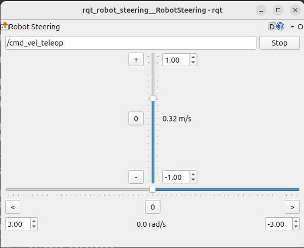
Stop the robot, by clicking the Stop button.
Close the rqt_robot_steering tool by pressing CTRL + C.
Cancel Assisted Teleoperation
To cancel assisted teleoperation, publish a cancellation message:
ros2 topic pub /cancel_assisted_teleop std_msgs/Bool "data: true" --onceTo restart assisted teleoperation, launch the rqt_robot_steering tool again, and move the sliders:
rqt_robot_steeringPress CTRL + C to close these nodes when you are done.
In this tutorial, we explored the Nav2 Simple Commander API and implemented various navigation functionalities for our robot, including basic goal navigation, predefined locations, and assisted teleoperation. You can find other code examples here at the Nav2 GitHub.
These implementations demonstrate the versatility of Nav2, combining autonomous navigation with user input for flexible control in various scenarios. The skills you’ve gained form a strong foundation for developing more complex robotic systems, applicable to real-world robots with minimal modifications.