
In this tutorial, we’ll learn how to convert camera pixel coordinates to coordinates that are relative to the base frame for a robotic arm.
Prerequisites
This tutorial will make a lot more sense if you’ve gone through the following tutorials first. Otherwise, if you are already familiar with terms like “homogeneous transformation matrix,” jump right ahead into this tutorial.
- You completed this tutorial to build a two degree of freedom robotic arm.
- You know how to draw the kinematic diagram for a two degree of freedom robotic arm.
- You know how to draw Denavit-Hartenberg Frames for a two degree of freedom robotic arm.
- You understand what homogeneous transformation matrices are and how to write them in code.
- You know how to find rotation matrices between coordinate frames.
- You know how to find displacement vectors between coordinate frames.
- You know how to convert camera pixels to real-world (centimeter) coordinates.
Case 1: Camera Lens is Parallel to the Surface
Label the Axes
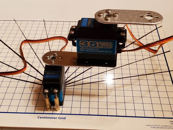
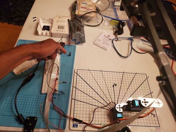
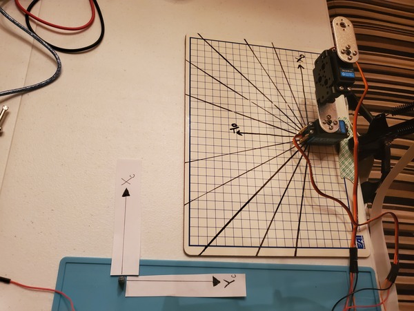
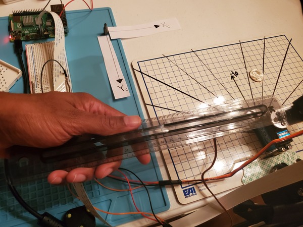
Here is a two degree of freedom robotic arm that I built.
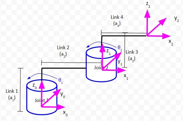
Here is the diagram of this robotic arm.
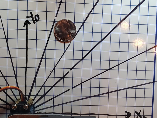
What we need to do is to draw the frames on the dry-erase board.
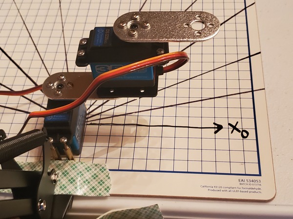
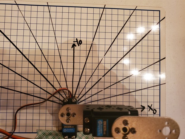
The origin of the base frame of the robotic arm is located here.
The x0 axis is this line here.
The y0 axis is this line here.
Open up your Raspberry Pi and turn on the video stream by running the following code:
# Credit: Adrian Rosebrock
# https://www.pyimagesearch.com/2015/03/30/accessing-the-raspberry-pi-camera-with-opencv-and-python/

# import the necessary packages
from picamera.array import PiRGBArray # Generates a 3D RGB array
from picamera import PiCamera # Provides a Python interface for the RPi Camera Module
import time # Provides time-related functions
import cv2 # OpenCV library

# Initialize the camera
camera = PiCamera()

# Set the camera resolution
camera.resolution = (640, 480)

# Set the number of frames per second
camera.framerate = 32

# Generates a 3D RGB array and stores it in rawCapture
raw_capture = PiRGBArray(camera, size=(640, 480))

# Wait a certain number of seconds to allow the camera time to warmup
time.sleep(0.1)

# Capture frames continuously from the camera
for frame in camera.capture_continuous(raw_capture, format="bgr", use_video_port=True):

    # Grab the raw NumPy array representing the image
    image = frame.array

    # Display the frame using OpenCV
    cv2.imshow("Frame", image)

    # Wait for keyPress for 1 millisecond
    key = cv2.waitKey(1) & 0xFF

    # Clear the stream in preparation for the next frame
    raw_capture.truncate(0)

    # If the `q` key was pressed, break from the loop
    if key == ord("q"):
        break
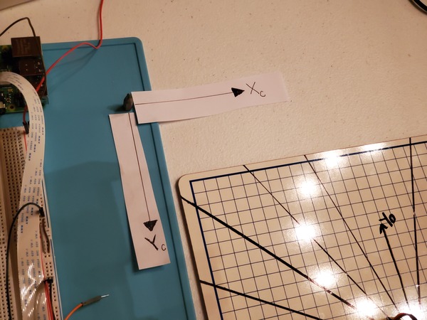
Let’s label the origin for the camera reference frame. The origin (x = 0, y = 0) for the camera reference frame is located in the far upper-left corner of the screen. I’ve put a screw driver head on the table to mark the location of the origin of the camera frame.
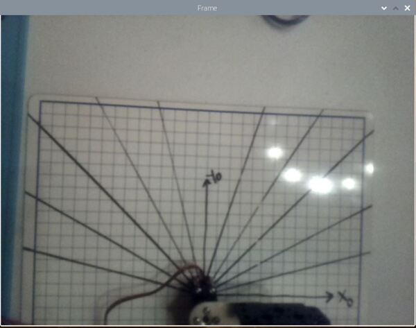
The x axis for the camera frame runs to the right from the origin along the top of the field of view. I’ll label this axis xc.
The y axis for the camera frame runs downward from the origin along the left side of the field of view. I’ll label this axis yc.
Press CTRL + C to stop the code from running.
Run the Object Detector Code
Run this code (absolute_difference_method_cm.py):
# Author: Addison Sears-Collins
# Description: This algorithm detects objects in a video stream
#   using the Absolute Difference Method. The idea behind this
#   algorithm is that we first take a snapshot of the background.
#   We then identify changes by taking the absolute difference
#   between the current video frame and that original
#   snapshot of the background (i.e. first frame).

# import the necessary packages
from picamera.array import PiRGBArray # Generates a 3D RGB array
from picamera import PiCamera # Provides a Python interface for the RPi Camera Module
import time # Provides time-related functions
import cv2 # OpenCV library
import numpy as np # Import NumPy library

# Initialize the camera
camera = PiCamera()

# Set the camera resolution
camera.resolution = (640, 480)

# Set the number of frames per second
camera.framerate = 30

# Generates a 3D RGB array and stores it in rawCapture
raw_capture = PiRGBArray(camera, size=(640, 480))

# Wait a certain number of seconds to allow the camera time to warmup
time.sleep(0.1)

# Initialize the first frame of the video stream
first_frame = None

# Create kernel for morphological operation. You can tweak
# the dimensions of the kernel.
# e.g. instead of 20, 20, you can try 30, 30
kernel = np.ones((20,20),np.uint8)

# Centimeter to pixel conversion factor
# I measured 32.0 cm across the width of the field of view of the camera.
CM_TO_PIXEL = 32.0 / 640

# Capture frames continuously from the camera
for frame in camera.capture_continuous(raw_capture, format="bgr", use_video_port=True):

    # Grab the raw NumPy array representing the image
    image = frame.array

    # Convert the image to grayscale
    gray = cv2.cvtColor(image, cv2.COLOR_BGR2GRAY)

    # Close gaps using closing
    gray = cv2.morphologyEx(gray,cv2.MORPH_CLOSE,kernel)

    # Remove salt and pepper noise with a median filter
    gray = cv2.medianBlur(gray,5)

    # If first frame, we need to initialize it.
    if first_frame is None:

      first_frame = gray

      # Clear the stream in preparation for the next frame
      raw_capture.truncate(0)

      # Go to top of for loop
      continue

    # Calculate the absolute difference between the current frame
    # and the first frame
    absolute_difference = cv2.absdiff(first_frame, gray)

    # If a pixel is less than ##, it is considered black (background).
    # Otherwise, it is white (foreground). 255 is upper limit.
    # Modify the number after absolute_difference as you see fit.
    _, absolute_difference = cv2.threshold(absolute_difference, 50, 255, cv2.THRESH_BINARY)

    # Find the contours of the object inside the binary image
    contours, hierarchy = cv2.findContours(absolute_difference,cv2.RETR_TREE,cv2.CHAIN_APPROX_SIMPLE)[-2:]
    areas = [cv2.contourArea(c) for c in contours]

    # If there are no countours
    if len(areas) < 1:

      # Display the resulting frame
      cv2.imshow('Frame',image)

      # Wait for keyPress for 1 millisecond
      key = cv2.waitKey(1) & 0xFF

      # Clear the stream in preparation for the next frame
      raw_capture.truncate(0)

      # If "q" is pressed on the keyboard,
      # exit this loop
      if key == ord("q"):
        break

      # Go to the top of the for loop
      continue

    else:

      # Find the largest moving object in the image
      max_index = np.argmax(areas)

    # Draw the bounding box
    cnt = contours[max_index]
    x,y,w,h = cv2.boundingRect(cnt)
    cv2.rectangle(image,(x,y),(x+w,y+h),(0,255,0),3)

    # Draw circle in the center of the bounding box
    x2 = x + int(w/2)
    y2 = y + int(h/2)
    cv2.circle(image,(x2,y2),4,(0,255,0),-1)

    # Calculate the center of the bounding box in centimeter coordinates
    # instead of pixel coordinates
    x2_cm = x2 * CM_TO_PIXEL
    y2_cm = y2 * CM_TO_PIXEL

    # Print the centroid coordinates (we'll use the center of the
    # bounding box) on the image
    text = "x: " + str(x2_cm) + ", y: " + str(y2_cm)
    cv2.putText(image, text, (x2 - 10, y2 - 10),
      cv2.FONT_HERSHEY_SIMPLEX, 0.5, (0, 255, 0), 2)

    # Display the resulting frame
    cv2.imshow("Frame",image)

    # Wait for keyPress for 1 millisecond
    key = cv2.waitKey(1) & 0xFF

    # Clear the stream in preparation for the next frame
    raw_capture.truncate(0)

    # If "q" is pressed on the keyboard,
    # exit this loop
    if key == ord("q"):
      break

# Close down windows
cv2.destroyAllWindows()
Now, grab an object. I’ll grab a quarter and place it in the field of view.
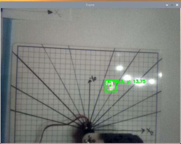
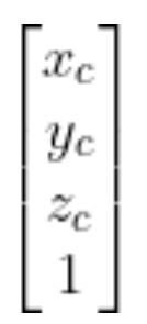
You can see the position of the quarter in the camera reference frame is:
- xc in centimeters = 19.5 cm
- yc in centimeters = 13.75 cm
- zc in centimeters = 0.0 cm
Finding the Homogeneous Transformation Matrix
This is cool, but what I really want to know are the coordinates of the quarter relative to the base frame of my two degree of freedom robotic arm.
If I know the coordinates of the object relative to the base frame of my two degree of freedom robotic arm, I can then use inverse kinematics to command the robot to move the end effector to that location.
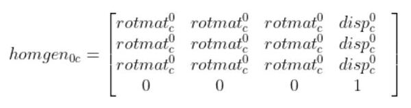
A tool that can help us do that is known as the homogeneous transformation matrix.
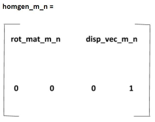
A homogeneous transformation matrix is a 4×4 matrix (i.e. 4 rows and 4 columns) that enables us to find the position of a point in reference frame m (e.g. the robotic arm base frame) given the position of a point in reference frame n (e.g. the camera reference frame).
In other words:
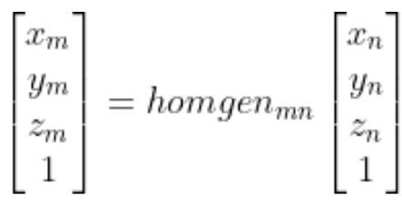
More, specifically:
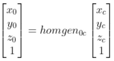
Which is the same thing as…
So you can see that if we know the vector:
If we can then determine the 4×4 matrix…
…and multiply the two terms together, We can calculate…
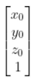
the position of the object in the robotic arm base reference frame.
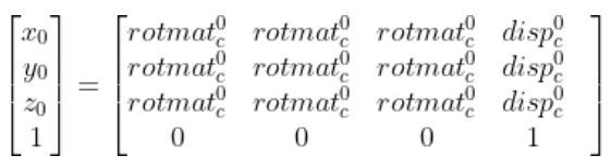
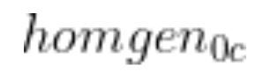
homgen0c has two pieces we need to find. We need to find the rotation matrix portion (i.e. the 3×3 matrix on the left. We also need to find the displacement vector portion (the rightmost column).
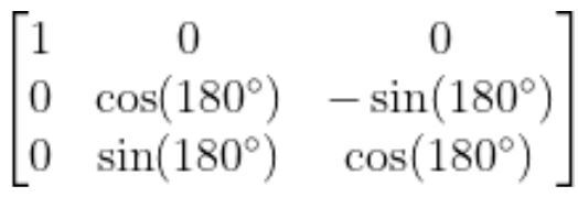
Calculate the Rotation Matrix That Converts the Camera Reference Frame to the Base Frame
Let’s start by finding the rotation matrix portion. I’m going to draw the camera and robotic base reference frames below. We first need to look at how we can rotate the base frame to match up with the camera frame of the robotic arm.
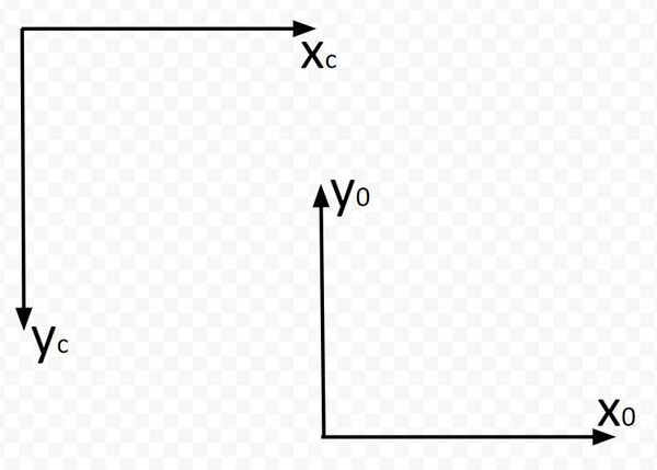
Which way is z0 pointing? Using the right hand rule, take your four fingers and point them towards the x0 axis. Your palm faces towards y0. Your thumb points towards z0, which is upwards out of the page (or upwards out of the dry erase board). I’ll mark this with a dark circle.
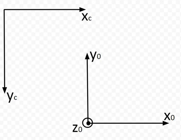
Which way is zc pointing? Using the right hand rule, take your four fingers and point them towards the xc axis. Your palm faces towards yc. Your thumb points towards zc, which is downwards into the page (or downward into the dry erase board). I’m marking this with an X.
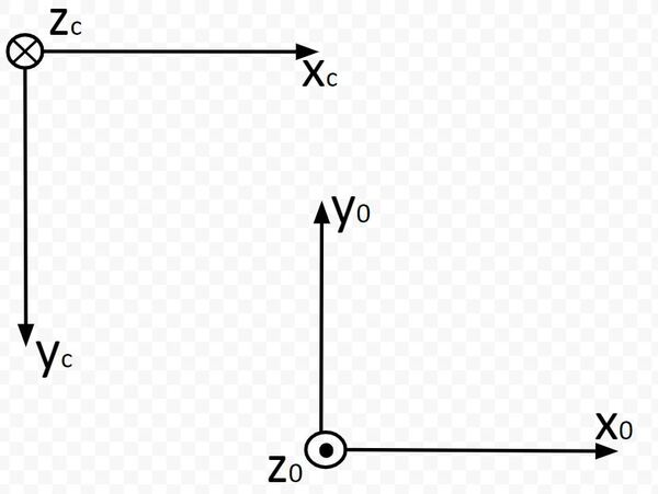
Now, stick your thumb in the direction of x0. Your thumb points is the axis of rotation, while your four fingers indicate the direction of positive rotation. You can see that we would need to rotate frame 0 an angle of +180 degrees around the x0 axis in order to get frame 0 to match up with frame c (the camera reference frame).
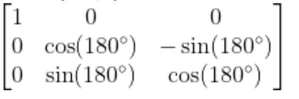
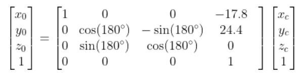
The standard rotation matrix for rotation around the x-axis is…
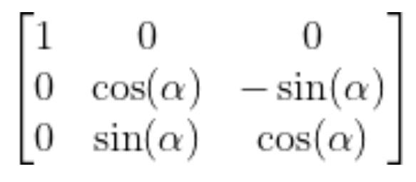
Substitute 180 degrees for ɑ, we get:
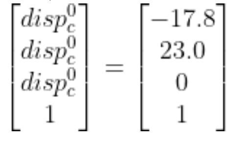
Calculate the Displacement Vector
Now that we have the rotation matrix portion of the homogeneous transformation matrix, we need to calculate the displacement vector from the origin of frame 0 to the origin of frame c.
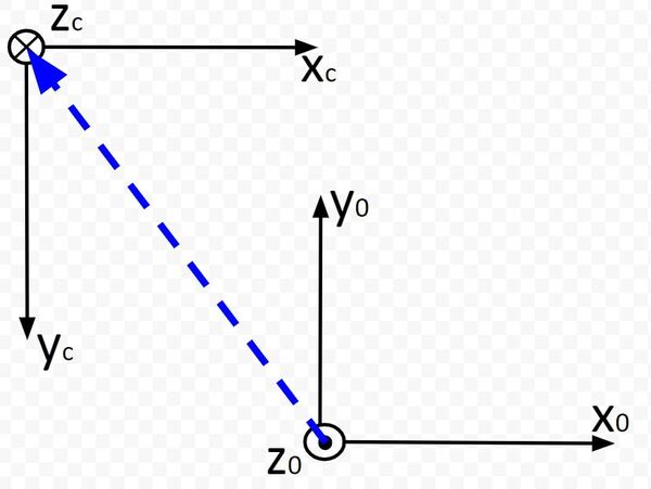
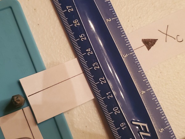
Displacement Along x0
Grab your ruler and measure the distance from the origin of frame 0 to the origin of frame c along the x0 axis.
I measured -17.8 cm (because the displacement is in the negative x0 direction).
Displacement Along y0
Grab your ruler and measure the distance from the origin of frame 0 to the origin of frame c along the y0 axis.
I measured 23.0 cm.
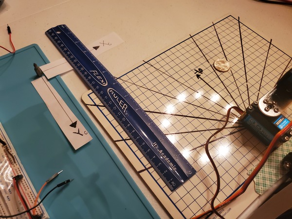
Displacement Along z0
Both reference frames are in the same z plane, so there is no displacement along z0 from frame 0 to frame c.
Therefore, we have 0.0 cm.
The full displacement vector is:
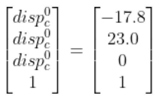
Putting It All Together
Now that we have our rotation matrix…
and our displacement vector…
we put them both together to get the following homogeneous transformation matrix.
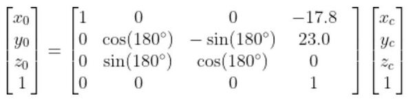
We can now convert a point in the camera reference frame to a point in the base frame of the robotic arm.
Print the Base Frame Coordinates of an Object
Now, let’s modify our absolute_difference_method_cm.py program so that we display an object’s x and y position in base frame coordinates rather than camera frame coordinates. I remeasured the width of the field of view in centimeters and calculated it as 36.0 cm.
I’ll name the program display_base_frame_coordinates.py.
Here is the code:
# Author: Addison Sears-Collins
# Description: This algorithm detects objects in a video stream
# using the Absolute Difference Method. The idea behind this
# algorithm is that we first take a snapshot of the background.
# We then identify changes by taking the absolute difference
# between the current video frame and that original
# snapshot of the background (i.e. first frame).
# The coordinates of an object are displayed relative to
# the base frame of a two degree of freedom robotic arm.
# import the necessary packages
from picamera.array import PiRGBArray # Generates a 3D RGB array
from picamera import PiCamera # Provides a Python interface for the RPi Camera Module
import time # Provides time-related functions
import cv2 # OpenCV library
import numpy as np # Import NumPy library
# Initialize the camera
camera = PiCamera()
# Set the camera resolution
camera.resolution = (640, 480)
# Set the number of frames per second
camera.framerate = 30
# Generates a 3D RGB array and stores it in rawCapture
raw_capture = PiRGBArray(camera, size=(640, 480))
# Wait a certain number of seconds to allow the camera time to warmup
time.sleep(0.1)
# Initialize the first frame of the video stream
first_frame = None
# Create kernel for morphological operation. You can tweak
# the dimensions of the kernel.
# e.g. instead of 20, 20, you can try 30, 30
kernel = np.ones((20,20),np.uint8)
# Centimeter to pixel conversion factor
# I measured 36.0 cm across the width of the field of view of the camera.
CM_TO_PIXEL = 36.0 / 640
# Define the rotation matrix from the robotic base frame (frame 0)
# to the camera frame (frame c).
rot_angle = 180 # angle between axes in degrees
rot_angle = np.deg2rad(rot_angle)
rot_mat_0_c = np.array([[1, 0, 0],
[0, np.cos(rot_angle), -np.sin(rot_angle)],
[0, np.sin(rot_angle), np.cos(rot_angle)]])
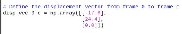
# Define the displacement vector from frame 0 to frame c
disp_vec_0_c = np.array([[-17.8],
[24.4], # This was originally 23.0 but I modified it for accuracy
[0.0]])
# Row vector for bottom of homogeneous transformation matrix
extra_row_homgen = np.array([[0, 0, 0, 1]])
# Create the homogeneous transformation matrix from frame 0 to frame c
homgen_0_c = np.concatenate((rot_mat_0_c, disp_vec_0_c), axis=1) # side by side
homgen_0_c = np.concatenate((homgen_0_c, extra_row_homgen), axis=0) # one above the other
# Initialize coordinates in the robotic base frame
coord_base_frame = np.array([[0.0],
[0.0],
[0.0],
[1]])
# Capture frames continuously from the camera
for frame in camera.capture_continuous(raw_capture, format="bgr", use_video_port=True):
# Grab the raw NumPy array representing the image
image = frame.array
# Convert the image to grayscale
gray = cv2.cvtColor(image, cv2.COLOR_BGR2GRAY)
# Close gaps using closing
gray = cv2.morphologyEx(gray,cv2.MORPH_CLOSE,kernel)
# Remove salt and pepper noise with a median filter
gray = cv2.medianBlur(gray,5)
# If first frame, we need to initialize it.
if first_frame is None:
first_frame = gray
# Clear the stream in preparation for the next frame
raw_capture.truncate(0)
# Go to top of for loop
continue
# Calculate the absolute difference between the current frame
# and the first frame
absolute_difference = cv2.absdiff(first_frame, gray)
# If a pixel is less than ##, it is considered black (background).
# Otherwise, it is white (foreground). 255 is upper limit.
# Modify the number after absolute_difference as you see fit.
_, absolute_difference = cv2.threshold(absolute_difference, 95, 255, cv2.THRESH_BINARY)
# Find the contours of the object inside the binary image
contours, hierarchy = cv2.findContours(absolute_difference,cv2.RETR_TREE,cv2.CHAIN_APPROX_SIMPLE)[-2:]
areas = [cv2.contourArea(c) for c in contours]
# If there are no countours
if len(areas) < 1:
# Display the resulting frame
cv2.imshow('Frame',image)
# Wait for keyPress for 1 millisecond
key = cv2.waitKey(1) & 0xFF
# Clear the stream in preparation for the next frame
raw_capture.truncate(0)
# If "q" is pressed on the keyboard,
# exit this loop
if key == ord("q"):
break
# Go to the top of the for loop
continue
else:
# Find the largest moving object in the image
max_index = np.argmax(areas)
# Draw the bounding box
cnt = contours[max_index]
x,y,w,h = cv2.boundingRect(cnt)
cv2.rectangle(image,(x,y),(x+w,y+h),(0,255,0),3)
# Draw circle in the center of the bounding box
x2 = x + int(w/2)
y2 = y + int(h/2)
cv2.circle(image,(x2,y2),4,(0,255,0),-1)
# Calculate the center of the bounding box in centimeter coordinates
# instead of pixel coordinates
x2_cm = x2 * CM_TO_PIXEL
y2_cm = y2 * CM_TO_PIXEL
# Coordinates of the object in the camera reference frame
cam_ref_coord = np.array([[x2_cm],
[y2_cm],
[0.0],
[1]])
# Coordinates of the object in base reference frame
coord_base_frame = homgen_0_c @ cam_ref_coord
# Print the centroid coordinates (we'll use the center of the
# bounding box) on the image
text = "x: " + str(coord_base_frame[0][0]) + ", y: " + str(coord_base_frame[1][0])
cv2.putText(image, text, (x2 - 10, y2 - 10),
cv2.FONT_HERSHEY_SIMPLEX, 0.5, (0, 255, 0), 2)
# Display the resulting frame
cv2.imshow("Frame",image)
# Wait for keyPress for 1 millisecond
key = cv2.waitKey(1) & 0xFF
# Clear the stream in preparation for the next frame
raw_capture.truncate(0)
# If "q" is pressed on the keyboard,
# exit this loop
if key == ord("q"):
break
# Close down windows
cv2.destroyAllWindows()
Run the code.
Then place a quarter on the dry erase board. You should see that the x and y coordinates of the quarter relative to the base frame are printed to the screen.
Then place a quarter on the dry erase board. You should see that the x and y coordinates of the quarter relative to the base frame are printed to the screen.
I am placing the quarter at x = 4 and y = 9. The text on the screen should now display the coordinates of the quarter in the base frame coordinates.
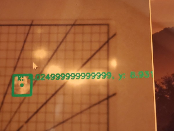
The first time I ran this code, my x coordinate was accurate, but my y coordinate was not. I modified the y displacement value until I got something in the ballpark of x =4 and y = 9 for the coordinates printed to the screen. In the end, my displacement value was 24.4 cm instead of 23.0 cm (which is what it was originally).
Thus, here was my final equation for converting camera coordinates to robotic base frame coordinates:
Where z0 = zc = 0 cm.
Pretty cool!
Case 2: Camera Lens Is Not Parallel To the Surface
Up until now, we have assumed that the camera lens is always parallel to the underlying surface like this.
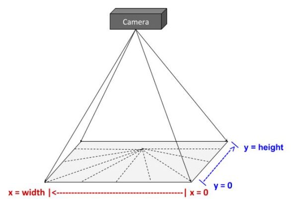
What happens if it isn’t, and instead the camera lens is looking down on the surface at some angle. You can imagine that in the real world, this situation is quite common.
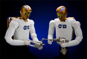
Consider this humanoid robot for example. This robot might have some sort of camera inside his helmet. Any surface that he looks at that is in front of his body will likely be from some angle.
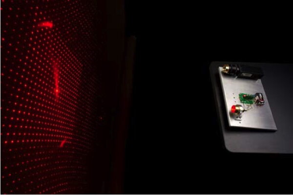
Also, in real-world use cases, a physical grid is usually not present. Instead, the structured light technique is used to project a known grid pattern on a surface in order to help the robot determine the coordinates of an object.
You can see an example of structured light developed at the NASA Jet Propulsion Laboratory on the left side of this image.
A robot that looks at structured light would also see it from an angle. So, what changes in this case?
Previously in this tutorial, we assumed that the pixel-to-centimeter conversion factor will be the same in the x and y directions. This assumption only holds true, however, if the camera lens is directly overhead and parallel to the grid surface. This all changes when the camera is looking at a surface from an angle.
One way we can solve this problem is to derive (based on observation) a function that takes as input the pixel coordinates of an object (as seen by the camera) and outputs the (x0,y0) real-world coordinates in centimeters (i.e. the robotic arm base frame).
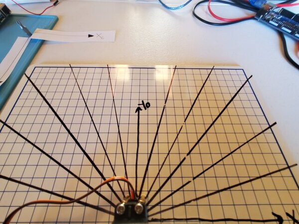
If you look at the image below, you can see that the pixel-to-centimeter conversion factor in the y (and x) direction is larger at the bottom of the image than it is at the top. And since the squares on the dry-erase board look more like rectangles, you know that the pixel-to-centimeter conversion factor is different in the x (horizontal) and y directions (vertical).
Example
Let’s do a real example, so you can see how to do this.
Create an Equation to Map Camera Pixel Y Coordinates to Global Reference Frame Y Coordinates in Centimeters
Open a snapshot from the tilted camera frame in a photo editing program like Microsoft Paint. My image is 640 pixels wide and 480 pixels in height.
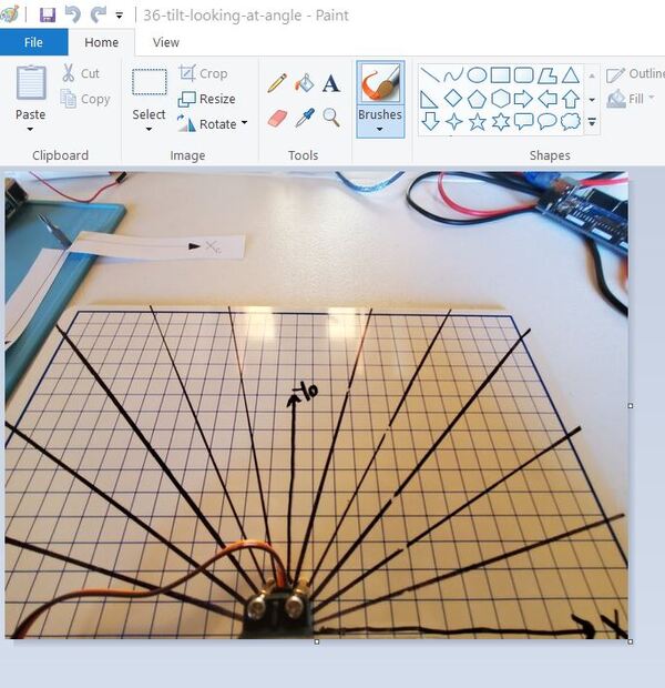
You can see in the bottom-left of Microsoft Paint how the program spits out the pixel location of my cursor. Make sure that whatever photo editing program you’re using gives you the ability to see pixel locations.
Open a blank spreadsheet. I’m using Microsoft Excel.
Create four columns:
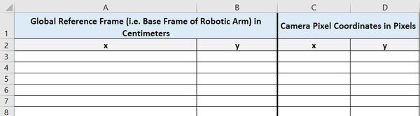
- x in Column A (Global Reference Frame coordinates in cm)
- y in Column B (Global Reference Frame coordinates in cm)
- x in Column A (Camera Pixel coordinates)
- y in Column B (Camera Pixel coordinates)
We will start by making x=0 and then finding the corresponding y.
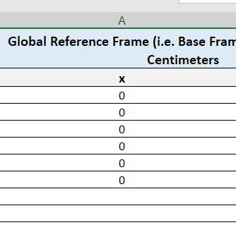
Let’s fill in y with some evenly spaced values.
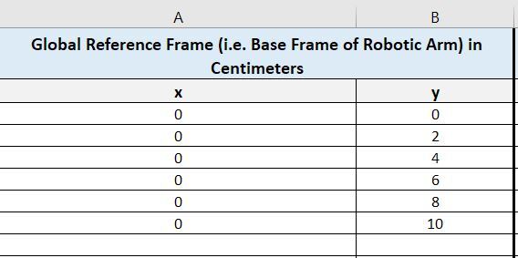
Take your cursor and place it on top of each global reference frame coordinate, and record the corresponding pixel value.
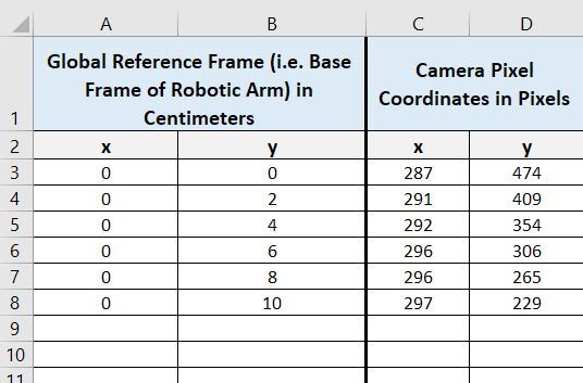
Now we want to find an equation that can convert camera pixel y coordinates to global reference frame y coordinates.
Plot the data. Here is how it looks.
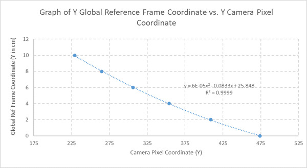
I will right-click on the data points and add a trendline. I will place a checkmark near the “Display Equation on chart” and “Display R-squared value” options. I want to have a good R-squared value. This value shows how well my trendline fits the data. The closer it is to 1, the better.
A Polynomial best-fit line of Order 2 gives me an R-squared value of around 0.9999, so let’s go with this equation.
(Global Reference Frame Y Coordinate in cm) = 0.00006*(Camera Pixel Y Coordinate)2 – 0.0833*(Camera Pixel Y Coordinate) + 25.848
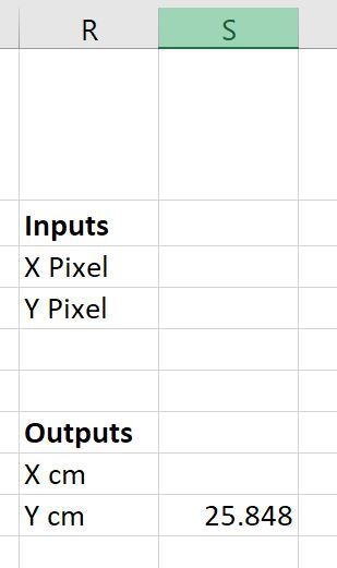
Now, let’s enter this formula into our spreadsheet.
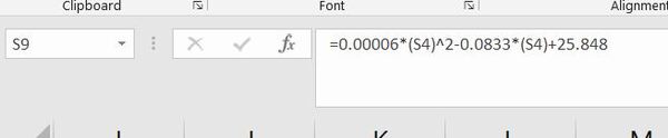
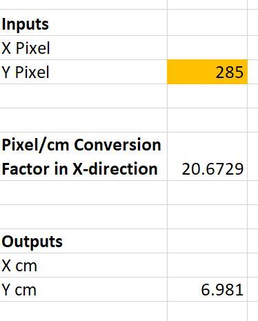
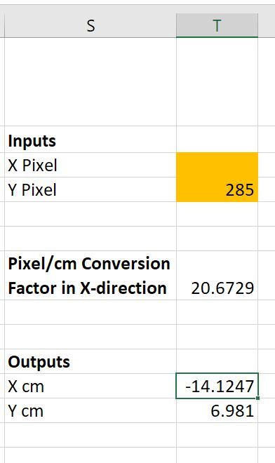
I’m going to test the equation by choosing a random y pixel value and seeing what the y coordinate would be in centimeters.
Go back to MS Paint. I’m going to put the cursor over (x=0 cm, y=7 cm) and then record what the y pixel value is.
I get a y pixel value of 285 when I put my cursor over this location. Let’s see what the equation spits out:
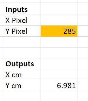
I calculated 6.981 cm. I expected to get a y value of 7 cm, so this is right around what I expected.
Create an Equation to Map Camera Pixel Y and X Coordinates to Global Reference Frame X Coordinates in Centimeters
Now let’s see how we can get the x position in centimeters. To do this, we need to do an interim step. Since the pixel-to-centimeter conversion factor in the x-direction varies along the y-axis, we need to find out the pixel-to-centimeter conversion factor in the x-direction for our original list of global reference frame y centimeter values.
Go to the spreadsheet and insert a column to the right of the Y values for the global reference frame. We will label this column Pixels per Centimeter.
Let’s start at y = 0 cm. The pixel value there for x is 287. Now, we go 1 cm over to the right (i.e. each square is 1 cm in length) and find an x pixel value of 316. Therefore, for y = 0 cm, the pixel-to-centimeter conversion factor in the x direction is:
(316 pixels – 287 pixels) / 1 cm = 29 pixels/cm
I’ll write that in the spreadsheet.
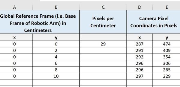
Now, do the same thing for all values of y in your spreadsheet.
Here is what my table now looks like:
Now what we want to do is create an equation that takes as input the global reference frame y value in centimeters and outputs the pixel-to-centimeter conversion factor along the x-direction.
Here is the plot of the data:
I will add a polynomial trendline of Order 2 and the R-squared value to see how well this line fits the data.
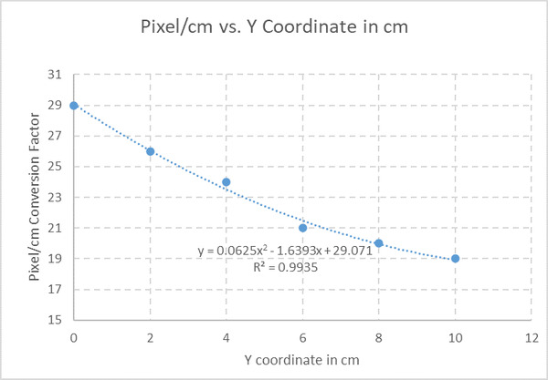
Our equation is:
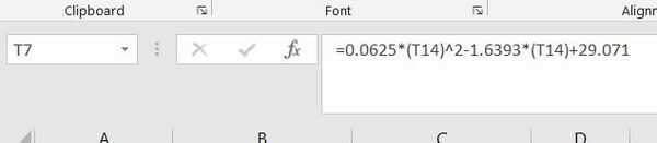
Pixel/cm Conversion Factor in the x-direction = 0.0625 * (Global Reference Frame Y Coordinate in cm)2 -1.6393 * (Global Reference Frame Y Coordinate in cm) + 29.071
Let’s add this to our spreadsheet.
Now to find the x position in centimeters of an object in the camera frame, we need to take the x position in pixels as input, subtract the x pixel position of the centerline (i.e. when ≈ 292 pixels…which is the average of the highest and lowest x pixel coordinates of the centerline) and then divide by the pixel-to-centimeter conversion factor (along the x-direction for the corresponding y cm position). In other words:
Global Reference Frame X Coordinate in cm = ((Camera Pixel X Coordinate) – (X Pixel Coordinate of the Centerline))/ (Pixel/cm Conversion Factor in the x-direction)
I will add this formula to the spreadsheet.
Putting It All Together
Let’s test our math out to see what we get.
Go over to MS Paint or whatever photo editor you’re using. Select a random point on the grid. I’ll select the point (x = 6 cm, y = 8 cm). MS Paint tells me that the pixel value at this location is: (x = 417 px, y = 265 px).
I’ll plug 417 and 265 into the spreadsheet as inputs.
You can see that our formula spit out:
- Global Reference Frame X Coordinate in cm: 6.26
- Global Reference Frame Y Coordinate in cm: 7.99
This result is pretty close to what we expected.
Congratulations! You now know what to do if you have a camera lens that is tilted relative to the plane of a gridded surface. No need to memorize this process. When you face this problem in the future, just come back to the steps I’ve outlined in this tutorial, and go through them one-by-one.
That’s it for this tutorial. Keep building!
References
Credit to Professor Angela Sodemann for teaching me this stuff. Dr. Sodemann is an excellent teacher (She runs a course on RoboGrok.com).