In this tutorial, we will create a basic “Hello World” project to get your feet wet with C++ and MoveIt 2. I will show you how to move the end of the robotic arm (where the gripper is located) to a desired position and orientation. 

The official instructions are on this page, but we will walk through everything together, step by step.

By the end of this tutorial, you will be able to create this:

Prerequisites

• You have completed this tutorial.

All my code for this project is located here on GitHub.

Create a Package

Let’s start by creating a new package for our project. Open a terminal and navigate to the mycobot_ros2 directory in your ROS 2 workspace:

cd ~/ros2_ws/src/mycobot_ros2/

Now, let’s create a new package using the ROS 2 command line tools:

ros2 pkg create --build-type ament_cmake --dependencies moveit_ros_planning_interface rclcpp --node-name hello_moveit_v1 --license BSD-3-Clause hello_moveit

This command creates a new package named “hello_moveit” with the necessary dependencies and a node named “hello_moveit_v1”. The package will be created inside the mycobot_ros2 directory.

Next, let’s move into our newly created package:

cd hello_moveit

Create a ROS Node and Executor

Now that we have our package in place, let’s set up our C++ file to work with MoveIt 2. We’ll start by editing the main source file.

Open the new source code file you created.

cd src

gedit hello_moveit_v1.cpp

Replace the existing content with the following code:

/**
 * @file hello_moveit_v1.cpp
 * @brief A simple program that sets up a ROS 2 node to work with MoveIt for robot control.
 *
 * This program creates a basic setup for controlling a robot using ROS 2 and MoveIt.
 * It doesn't actually move the robot yet, but it prepares everything we need to start
 * planning robot movements in future steps.
 *
 * @author Addison Sears-COllins
 * @date August 07, 2024
 */

#include <memory>
#include <rclcpp/rclcpp.hpp>
#include <moveit/move_group_interface/move_group_interface.h>

/**
 * @brief The main function that starts our program.
 *
 * This function sets up our ROS 2 environment and prepares it for robot control.
 *
 * @param argc The number of input arguments our program receives.
 * @param argv The list of input arguments our program receives.
 * @return int A number indicating if our program finished successfully (0) or not.
 */
int main(int argc, char * argv[])
{
  // Start up ROS 2
  rclcpp::init(argc, argv);
  
  // Creates a node named "hello_moveit". The node is set up to automatically
  // handle any settings (parameters) we might want to change later without editing the code.
  auto const node = std::make_shared<rclcpp::Node>(
    "hello_moveit",
    rclcpp::NodeOptions().automatically_declare_parameters_from_overrides(true)
  );

  // Creates a "logger" that we can use to print out information or error messages
  // as our program runs.
  auto const logger = rclcpp::get_logger("hello_moveit");

  // We'll add code here later to actually plan robot movements
  RCLCPP_INFO(logger, "We'll add code here later to actually plan robot movements");

  // Shut down ROS 2 cleanly when we're done
  rclcpp::shutdown();
  return 0;
}

This code sets up the basic structure we need to work with MoveIt 2. It initializes ROS 2, creates a node, sets up logging, and creates a MoveGroupInterface for our robot’s arm.

Let’s compile our code to make sure everything is set up correctly. Go back to your workspace directory:

cd ~/ros2_ws

To build the package with debug information, we’ll use the following command:

colcon build --packages-select hello_moveit

This command builds only our hello_moveit package.

After the build completes successfully, open a new terminal and source your workspace:

source ~/.bashrc

Now you can run your program:

ros2 run hello_moveit hello_moveit_v1

At this point, the program should run and exit without any errors, though it won’t perform any robot movements yet. This step simply confirms that our basic setup is working correctly.

Plan and Execute Using MoveGroupInterface

Now that we’ve confirmed our basic setup is working, let’s add the code to plan and execute a motion for our robotic arm. 

Create a new file called hello_moveit_v2.cpp

cd ~/ros2_ws/src/mycobot_ros2/hello_moveit/src

gedit hello_moveit_v2.cpp

Add the following code:

/**
 * @file hello_moveit_v2.cpp
 * @brief A simple ROS 2 and MoveIt 2 program to control a robot arm
 *
 * This program demonstrates how to use ROS 2 and MoveIt 2 to control a robot arm.
 * It sets up a node, creates a MoveGroupInterface for the arm, sets a target pose for the gripper_base,
 * plans a trajectory, and executes the planned motion.
 *
 * @author Addison Sears-Collins
 * @date August 07, 2024
 */

#include <geometry_msgs/msg/pose_stamped.hpp>
#include <memory>
#include <rclcpp/rclcpp.hpp>
#include <moveit/move_group_interface/move_group_interface.h>

/**
 * @brief The main function that starts our program.
 *
 * This function sets up our ROS 2 environment and prepares it for robot control.
 *
 * @param argc The number of input arguments our program receives.
 * @param argv The list of input arguments our program receives.
 * @return int A number indicating if our program finished successfully (0) or not.
 */
int main(int argc, char * argv[])
{
  // Start up ROS 2
  rclcpp::init(argc, argv);
  
  // Creates a node named "hello_moveit". The node is set up to automatically
  // handle any settings (parameters) we might want to change later without editing the code.
  auto const node = std::make_shared<rclcpp::Node>(
    "hello_moveit",
    rclcpp::NodeOptions().automatically_declare_parameters_from_overrides(true)
  );

  // Creates a "logger" that we can use to print out information or error messages
  // as our program runs.
  auto const logger = rclcpp::get_logger("hello_moveit");

  // Create the MoveIt MoveGroup Interfaces
  // These interfaces are used to plan and execute movements, set target poses,
  // and perform other motion-related tasks for each respective part of the robot.
  // The use of auto allows the compiler to automatically deduce the type of variable.
  // Source: https://github.com/moveit/moveit2/blob/main/moveit_ros/planning_interface/move_group_interface/include/moveit/move_group_interface/move_group_interface.h
  using moveit::planning_interface::MoveGroupInterface;
  auto arm_group_interface = MoveGroupInterface(node, "arm");

  // Specify a planning pipeline to be used for further planning 
  arm_group_interface.setPlanningPipelineId("ompl");
  
  // Specify a planner to be used for further planning
  arm_group_interface.setPlannerId("RRTConnectkConfigDefault");  

  // Specify the maximum amount of time in seconds to use when planning
  arm_group_interface.setPlanningTime(1.0);
  
  // Set a scaling factor for optionally reducing the maximum joint velocity. Allowed values are in (0,1].
  arm_group_interface.setMaxVelocityScalingFactor(1.0);
  
  //  Set a scaling factor for optionally reducing the maximum joint acceleration. Allowed values are in (0,1].
  arm_group_interface.setMaxAccelerationScalingFactor(1.0);

  // Display helpful logging messages on the terminal
  RCLCPP_INFO(logger, "Planning pipeline: %s", arm_group_interface.getPlanningPipelineId().c_str());    
  RCLCPP_INFO(logger, "Planner ID: %s", arm_group_interface.getPlannerId().c_str());
  RCLCPP_INFO(logger, "Planning time: %.2f", arm_group_interface.getPlanningTime());

  // Set a target pose for the end effector of the arm 
  auto const arm_target_pose = [&node]{
    geometry_msgs::msg::PoseStamped msg;
    msg.header.frame_id = "base_link";
    msg.header.stamp = node->now(); 
    msg.pose.position.x = 0.061;
    msg.pose.position.y = -0.176;
    msg.pose.position.z = 0.168;
    msg.pose.orientation.x = 1.0;
    msg.pose.orientation.y = 0.0;
    msg.pose.orientation.z = 0.0;
    msg.pose.orientation.w = 0.0;
    return msg;
  }();
  arm_group_interface.setPoseTarget(arm_target_pose);

  // Create a plan to that target pose
  // This will give us two things:
  // 1. Whether the planning was successful (stored in 'success')
  // 2. The actual motion plan (stored in 'plan')
  auto const [success, plan] = [&arm_group_interface] {
    moveit::planning_interface::MoveGroupInterface::Plan msg;
    auto const ok = static_cast<bool>(arm_group_interface.plan(msg));
    return std::make_pair(ok, msg);
  }();

  // Try to execute the movement plan if it was created successfully
  // If the plan wasn't successful, report an error
  // Execute the plan
  if (success)
  {
    arm_group_interface.execute(plan);
  }
    else
  {
    RCLCPP_ERROR(logger, "Planning failed!");
  }
  
  // Shut down ROS 2 cleanly when we're done
  rclcpp::shutdown();
  return 0;
}

This code does the following:

1. Sets a target pose for the end effector (gripper_base) of the robotic arm.
2. Plans a path to reach that target pose.
3. Executes the plan if it was successful, or logs an error if planning failed.

Now, let’s build our updated code.

Go to CMakeLists.txt

cd ~/ros2_ws/src/mycobot_ros2/hello_moveit/

gedit CMakeLists.txt

Update the file with the hello_moveit_v2.cpp code.

Save the file, and close it.

cd ~/ros2_ws

colcon build

source ~/.bashrc

Launch the controller and Gazebo:

ros2 launch mycobot_gazebo mycobot_280_arduino_bringup_ros2_control_gazebo.launch.py use_rviz:=false

Start the MoveGroup with RViz.

ros2 launch mycobot_moveit_config_manual_setup move_group.launch.py

In another terminal, run your program to move the robotic arm from one place to another:

ros2 run hello_moveit hello_moveit_v2

You can safely ignore this warning:

[moveit_ros.robot_model_loader]: No kinematics plugins defined. Fill and load kinematics.yaml!

If everything is set up correctly, you should see the robot’s gripper move in RViz to the specified pose.

You can confirm the gripper is in the correct pose by typing the following command and comparing it to the pose you set in your hello_moveit_v2.cpp file.

ros2 run tf2_ros tf2_echo base_link gripper_base

Note: If you run the hello_moveit_v2 node without first launching the demo launch file, it will wait for 10 seconds and then exit with an error message. This is because the MoveGroupInterface looks for a node publishing the robot description topic, which is provided by the demo launch file.

Let’s break down the key components of our hello_moveit_v2.cpp file to understand how it works with MoveIt 2 for controlling the arm.

MoveGroupInterface Creation:

This part sets up a control interface for the robot’s arm. It’s like creating a special remote control that lets us send commands to move the arm.

Setting the Target Pose:

Here, we’re telling the arm where we want it to go. 

Planning the Motion:

This is where the robot figures out how to move from its current position to the target we set. It’s like planning a route on a map – the robot calculates all the steps needed to get from point A to point B safely.

Executing the Plan:

Finally, if the planning was successful, we tell the robot to actually perform the movement we planned. If the planning failed for some reason, we just report an error instead of trying to move.

These steps work together to allow us to control the robot arm in a safe and precise manner, moving it to exactly where we want it to go.

That’s it! Keep building.

In the previous tutorial, you learned how to leverage ROS 2 Control to move the robotic arm manually by sending raw joint commands to the robot. This exercise is great for learning, but it is not how things are done in a real-world robotics project.

In this tutorial, I will show you how to set up a ROS 2 software called MoveIt 2 to send those commands. MoveIt 2 is a powerful and flexible motion planning framework for robotic manipulators.

Using MoveIt 2 instead of sending manual commands through a terminal window allows for more sophisticated, efficient, and safer motion planning, taking into account obstacles, joint limits, and other constraints automatically.

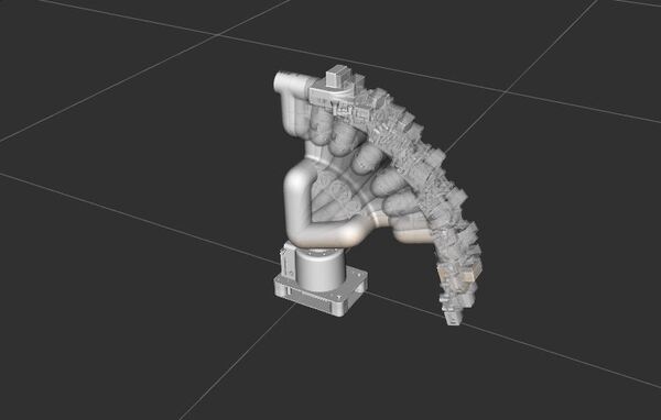
By the end of this tutorial, you will be able to create this:

Prerequisites

• You have completed my tutorial “How to Control a Robotic Arm Using ROS 2 Control and Gazebo.”
• I am working with ROS 2 Iron. Other ROS 2 distributions follow this similar process.

All my code for this project is located here on GitHub.

How MoveIt 2 Works with ROS 2 Control

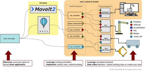
Before we dive into the tutorial, let me explain how MoveIt 2 works with ROS 2 Control by walking through a common real-world use case.

Suppose you have a mobile manipulator, which consists of a wheeled robot base with a robotic arm attached to it.

You want to develop an application that performs a pick and place task. 

Your cool app starts by telling MoveIt 2, “Pick up the object at location A and place it at location B.”

MoveIt 2, with help from Nav 2 (the navigation software stack for ROS 2), plans out the detailed movements needed – reaching for the object, grasping it, lifting it, moving to the new location, and placing it down.

These plans are sent to ROS 2 Control’s Controller Management system, which has specific controllers for the arm, gripper, and base.

The arm controller (e.g. JointTrajectoryController), for example, breaks down the plan into specific joint movements and sends these to the Resource Management system.

The Resource Management system communicates these commands through hardware interfaces to the actual robot parts (or their simulated versions).

As the robot executes the pick and place task, sensors in its joints and gripper send back information about position, force, and status.

This feedback flows back up through the system, allowing your app and MoveIt 2 to monitor progress and make adjustments if needed.

This setup allows you to focus on defining high-level tasks while MoveIt 2 and ROS 2 Control handle the complex details of robot control and movement coordination.

Now let’s look at another diagram which shows the specific controller and topic names. This gives us a more detailed view of how MoveIt 2, ROS 2 Control, and the robot components interact:

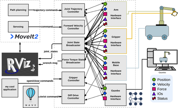
Your cool application initiates the process, defining tasks like pick and place operations.

MoveIt 2 contains a path planning component that generates trajectory commands. These commands are sent to the Joint Trajectory Controller, which manages the arm’s movements.

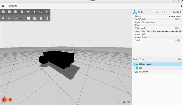
For mobile robots, Nav 2 can send twist commands to the Diff Drive Controller, controlling the base’s motion.

The system includes several specialized controllers:

• Joint Trajectory Controller for arm movements
• Forward Velocity Controller for speed control (optional…only needed if you need direct velocity control for high-speed operations)
• Gripper Controller for end-effector actions (e.g. open and close gripper)
• Diff Drive Controller for mobile base navigation

These controllers communicate with Hardware Interfaces for the arm, gripper, mobile base, and the Gazebo simulation.

As the robot operates, sensor data flows back through these Hardware Interfaces. This information includes position, velocity, force, and status updates.

The Joint State Broadcaster and Force Torque State Broadcaster collect this feedback data.

This state information (e.g. joint angles) is then forwarded to RViz for visualization and to MoveIt 2 for real-time monitoring and adjustment.

Create a Package

Now that you understand how all the pieces work together on a high level, let’s start setting up our robot with MoveIt 2.

Create a new package called mycobot_moveit_config_manual_setup:

cd ~/ros2_ws/src/mycobot_ros2/

ros2 pkg create --build-type ament_cmake --license BSD-3-Clause mycobot_moveit_config_manual_setup

cd mycobot_moveit_config_manual_setup

Fill in the package.xml file with your relevant information.

gedit package.xml

<?xml version="1.0"?>
<?xml-model href="http://download.ros.org/schema/package_format3.xsd" schematypens="http://www.w3.org/2001/XMLSchema"?>
<package format="3">
  <name>mycobot_moveit_config_manual_setup</name>
  <version>0.0.0</version>
  <description>Contains the files that enable the robot to integrate with Move It 2.</description>
  <maintainer email="automaticaddison@todo.com">Automatic Addison</maintainer>
  <license>BSD-3-Clause</license>

  <buildtool_depend>ament_cmake</buildtool_depend>
  
  <depend>moveit_ros_planning_interface</depend>
  <depend>moveit_ros_move_group</depend>
  <depend>moveit_kinematics</depend>
  <depend>moveit_planners_ompl</depend>
  <depend>moveit_ros_visualization</depend>
  <depend>rviz2</depend>
  <depend>rviz_visual_tools</depend> 

  <exec_depend>moveit_simple_controller_manager</exec_depend>
  <exec_depend>moveit_configs_utils</exec_depend>
  <exec_depend>pilz_industrial_motion_planner</exec_depend>

  <test_depend>ament_lint_auto</test_depend>
  <test_depend>ament_lint_common</test_depend>

  <export>
    <build_type>ament_cmake</build_type>
  </export>
</package>

Save the file, and close it.

In a real robotics project, the naming convention for this package would be:

<robot_name>_moveit_config

Create the Configuration Files

Let’s create configuration files that will enable us to tailor our robot for MoveIt 2. We’ll do this process manually first (recommended), and then we will work through how to do this using the MoveIt Setup Assistant. 

You can see some official examples of configuration files for other robots on the MoveIt resources ROS 2 GitHub.

Create the Config Folder

MoveIt 2 requires configuration files to go into the config folder of the package you created.

Open a terminal window, and type:

cd ~/ros2_ws/src/mycobot_ros2/mycobot_moveit_config_manual_setup/

mkdir config && cd config

Add SRDF

The first thing we need to do is set up the SRDF File. 

Semantic Robot Description Format (SRDF) is a file that tells MoveIt how your robot prefers to move and interact with its environment. It is a supplement to the URDF file.

The SRDF adds semantic (meaning-based) information to the robot’s description that isn’t included in the URDF (Unified Robot Description Format). This file includes things like:

• Naming groups of joints or links (e.g., “arm”, “gripper”)
• Defining default robot poses (e.g., “home”, “closed”, etc.)
• Which parts of the robot should be checked for colliding with each other during movement.
  • We need to do this step because checking every possible collision between all parts of the robot for each planned movement can be time-consuming, especially for complex robots.

cd ~/ros2_ws/src/mycobot_ros2/mycobot_moveit_config_manual_setup/config/

gedit mycobot_280.srdf

Add this code.

Save the file, and close it.

Let’s go through each section briefly:

1. <group name=”arm”>: This section defines a group named “arm” that includes a list of joints. The joints listed in this group represent the robot arm.
2. <group name=”gripper”>: This section defines a group named “gripper” that includes a list of joints related to the robot’s gripper or end-effector.
3. <group_state name=”home” group=”arm”>: This section defines a named state called “home” for the “arm” group. It specifies the joint values for the arm joints when the robot is in its home position.
4. <group_state name=”open” group=”gripper”>: This section defines a named state called “open” for the “gripper” group, specifying the joint value for the gripper when it is in its open position.
5. <disable_collisions>: This section is used to disable collision checking between specific pairs of links. Each <disable_collisions> entry specifies two links and the reason for disabling collision checking between them. The reasons can be “Adjacent” (for adjacent links in the robotic arm), “Never” (for links that will never collide), or “Default” (for links that are not expected to collide in most configurations).

Add Initial Positions

Now let’s create a configuration file for the initial positions.

cd ~/ros2_ws/src/mycobot_ros2/mycobot_moveit_config_manual_setup/config/

gedit initial_positions.yaml

Add this code.

# Default initial position for each movable joint
initial_positions:
  link1_to_link2: 0.0
  link2_to_link3: 0.0
  link3_to_link4: 0.0
  link4_to_link5: 0.0
  link5_to_link6: 0.0
  link6_to_link6flange: 0.0
  gripper_controller: 0.0

Save the file. This code sets the default initial positions for each movable joint. 

The initial_positions.yaml file in MoveIt specifies the starting joint positions for motion planning, overriding any default positions set in the URDF. It allows you to set a specific initial configuration for your robot in MoveIt without modifying the URDF, providing flexibility in defining the starting point for motion planning tasks.

Add Joint Limits

gedit joint_limits.yaml

Add this code.

default_velocity_scaling_factor: 1.0
default_acceleration_scaling_factor: 1.0

joint_limits:
  link1_to_link2:
    has_velocity_limits: true
    max_velocity: 2.792527
    has_acceleration_limits: true
    max_acceleration: 5.0
    has_deceleration_limits: true
    max_deceleration: -5.0
    has_jerk_limits: false
    max_jerk: 6.0
  link2_to_link3:
    has_velocity_limits: true
    max_velocity: 2.792527
    has_acceleration_limits: true
    max_acceleration: 5.0
    has_deceleration_limits: true
    max_deceleration: -5.0
    has_jerk_limits: false
    max_jerk: 6.0
  link3_to_link4:
    has_velocity_limits: true
    max_velocity: 2.792527
    has_acceleration_limits: true
    max_acceleration: 5.0
    has_deceleration_limits: true
    max_deceleration: -5.0
    has_jerk_limits: false
    max_jerk: 6.0
  link4_to_link5:
    has_velocity_limits: true
    max_velocity: 2.792527
    has_acceleration_limits: true
    max_acceleration: 5.0
    has_deceleration_limits: true
    max_deceleration: -5.0
    has_jerk_limits: false
    max_jerk: 6.0
  link5_to_link6:
    has_velocity_limits: true
    max_velocity: 2.792527
    has_acceleration_limits: true
    max_acceleration: 5.0
    has_deceleration_limits: true
    max_deceleration: -5.0
    has_jerk_limits: false
    max_jerk: 6.0
  link6_to_link6flange:
    has_velocity_limits: true
    max_velocity: 2.792527
    has_acceleration_limits: true
    max_acceleration: 5.0
    has_deceleration_limits: true
    max_deceleration: -5.0
    has_jerk_limits: false
    max_jerk: 6.0
  gripper_controller:
    has_velocity_limits: true
    max_velocity: 2.792527
    has_acceleration_limits: true
    max_acceleration: 5.0
    has_deceleration_limits: true
    max_deceleration: -5.0
    has_jerk_limits: false
    max_jerk: 300.0

Save the file.

This code sets the velocity and acceleration limits for each joint in our robotic arm, which is used by MoveIt 2 to control the robot’s movements.

Even though we have joint limits for velocity already defined in the URDF, this YAML file allows for overriding. Defining joint limits specific to MoveIt 2 is useful if you want to impose stricter or different limits for particular applications without modifying the URDF. It provides flexibility in adjusting the robot’s behavior for different tasks.

Add Kinematics

gedit kinematics.yaml

Add this code, and save the file. 

# Configures how a robot calculates possible positions and movements of its joints 
# to reach a desired point. It specifies which mathematical methods (solvers) to use, 
# how long to try, and how precise these calculations should be.
arm: # Name of the joint group from the SRDF file
  kinematics_solver: kdl_kinematics_plugin/KDLKinematicsPlugin # Plugin used for solving kinematics
  kinematics_solver_search_resolution: 0.005 #  Granularity (in radians for revolute joints) used by the solver when searching for a solution.
  kinematics_solver_timeout: 0.05 # Maximum time the solver will spend trying to find a solution for each planning attempt
  position_only_ik: false # If true, the solver will only consider the position of the end effector, not its orientation
  kinematics_solver_attempts: 5 # How many times the solver will try to find a solution

# Typically we don't need a complex kinematics solver for the gripper. This is for demonstration purposes only.  
gripper:
  kinematics_solver: kdl_kinematics_plugin/KDLKinematicsPlugin
  kinematics_solver_search_resolution: 0.005
  kinematics_solver_timeout: 0.05
  position_only_ik: false
  kinematics_solver_attempts: 3
  
arm_with_gripper:
  kinematics_solver: kdl_kinematics_plugin/KDLKinematicsPlugin
  kinematics_solver_search_resolution: 0.005
  kinematics_solver_timeout: 0.05
  position_only_ik: false
  kinematics_solver_attempts: 5

This file configures how MoveIt 2 calculates possible positions and movements of the robot’s arm to reach a desired point in space. It specifies the mathematical methods, precision, and time limits for these calculations, which MoveIt 2 uses to plan the robot’s movements.

Add Controllers

gedit moveit_controllers.yaml

Add this code, and save the file. 

# This file configures the controller management for MoveIt, specifying which controllers are available,
# the joints each controller handles, and the type of interface (e.g. FollowJointTrajectory).
moveit_controller_manager: moveit_simple_controller_manager/MoveItSimpleControllerManager  # Specifies the controller manager to use.

# Define the controllers configured using the ROS 2 Control framework.
moveit_simple_controller_manager:
  controller_names:
    - arm_controller   # Name of the controller for the robotic arm.
    - grip_controller  # Name of the controller for the gripper.
    - grip_action_controller # Other controller for the gripper (recommended)

  # Configuration for the arm_controller.
  arm_controller:
    action_ns: follow_joint_trajectory   # ROS action namespace to which MoveIt sends trajectory commands.
    type: FollowJointTrajectory          # Type of the controller interface; follows a joint trajectory.
    default: true                        # This controller is the default for the joints listed below.
    joints:                              # List of joints that the arm_controller manages.
      - link1_to_link2
      - link2_to_link3
      - link3_to_link4
      - link4_to_link5
      - link5_to_link6
      - link6_to_link6flange

  # Configuration for the grip_controller.
  grip_controller:
    action_ns: follow_joint_trajectory  
    type: FollowJointTrajectory         
    default: false                    
    joints:                           
      - gripper_controller      
  
  # Configuration for the grip_action_controller.    
  grip_action_controller:  
    action_ns: gripper_cmd 
    type: GripperCommand
    default: true
    joints:
      - gripper_controller       

This yaml file tells MoveIt 2 how to convert its motion plans into instructions that the ROS 2 controllers can understand and execute on the real (or simulated) robot. Without this, MoveIt 2 wouldn’t know how to make the robot actually move using the ROS 2 control system.

MoveIt 2 sends desired joint positions or trajectories to ROS 2 controllers, which then manage the low-level control of the robot’s motors. This integration allows MoveIt 2 to focus on high-level motion planning while relying on ROS 2 control for the actual execution on the robot hardware.

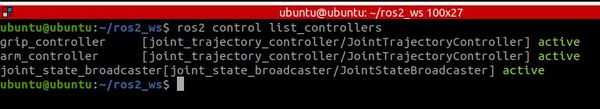
We see that three ROS 2 controllers are available:

• arm_controller: This is a Joint Trajectory Controller for the robot arm
• grip_controller: This is a Joint Trajectory Controller for the gripper (optional)
• grip_action_controller: This is a Gripper Action Controller for the gripper

We also see a list of joints associated with each controller.

The arm controller uses the “FollowJointTrajectory” action interface. The FollowJointTrajectory action interface is a standardized interface in ROS (Robot Operating System) for controlling the joint positions of a robot over time. It allows MoveIt 2 to send a trajectory, which is a sequence of joint positions and their corresponding timestamps, to the robot’s joint controllers.

How it works:

1. MoveIt 2 plans a movement, which results in a series of joint positions over time.
2. This plan is packaged into a “trajectory” – think of it as a list of goal positions (in radians) for each joint.
3. MoveIt 2 sends this trajectory to the appropriate ROS 2 controller using the FollowJointTrajectory action interface. This interface is like a protocol MoveIt 2 uses to communicate with the controllers.
4. The ROS 2 controller receives this trajectory, processes it, and relays it to the hardware interface.
5. The hardware interface sends the commands to the microcontroller (e.g. Arduino) to move the robot’s joints accordingly.

Add Cartesian Speed and Acceleration Limits

For motion planning for our robotic arm, we are going to use the Pilz industrial motion planner.

Pilz focuses on simple, predictable movements like straight lines, circles, and direct point-to-point paths. It works by calculating a clear, predefined route for each part of the robot to follow, ensuring smooth and safe motion from start to finish.

Think of Pilz as a careful driver that always takes known, reliable routes rather than trying to find creative shortcuts, making it perfect for precise tasks where you want consistent, controlled movements.

While default planners like OMPL (Open Motion Planning Library) work best for dynamic environments where you can have unexpected obstacles (people moving around, objects left on tabletops and counters, etc.), the structured and predictable nature of Pilz is advantageous in a scenario where the environment is well-structured and controlled.

Open a new file where we will define the Cartesian limits:

gedit pilz_cartesian_limits.yaml  

# Defines the Cartesian movement limits for a robotic arm using the Pilz Planner.
# The values are typically determined based on a combination of the robot manufacturer's 
# specifications, practical testing, and considerations for the specific tasks the robot will perform.
cartesian_limits:
  max_trans_vel: 1.0  # Maximum translational velocity in meters per second. Specifies how fast the end effector can move in space.
  max_trans_acc: 2.25 # Maximum translational acceleration in meters per second squared. Determines how quickly the end effector can increase its speed.
  max_trans_dec: -5.0 # Maximum translational deceleration in meters per second squared. Specifies how quickly the end effector can decrease its speed.
  max_rot_vel: 1.57   # Maximum rotational velocity in radians per second. Controls the speed at which the end effector can rotate.

Save the file, and close it.

This file sets speed and acceleration limits for a robotic arm’s movement in space. It defines how fast and quickly the robot’s end effector can move and rotate in Cartesian space (X, Y, Z direction) to ensure safe and efficient operation within the robot’s workspace.

Why do we need this file if we have already set velocity limits inside the URDF?

The URDF and the MoveIt configuration files serve different purposes when it comes to controlling the robot’s motion. The URDF contains velocity limits for each individual joint, which determine how fast each joint can move. These limits are important for controlling the speed of the individual joints. For example:

<joint name="joint_name" type="revolute">
  <limit lower="-2.879793" upper="2.879793" effort="5.0" velocity="2.792527"/>
</joint>

On the other hand, the cartesian_limits in the MoveIt configuration are used to control the speed and motion of the robot’s gripper in 3D space. These limits define how fast the gripper can move and rotate in the world coordinate frame (X, Y, Z axes). The cartesian_limits are essential for planning the overall motion of the robot and ensuring that it moves safely and efficiently when performing tasks.

So, while the URDF velocity limits are important for controlling individual joints, the MoveIt cartesian_limits are still necessary for proper motion planning and control of the gripper’s movement in 3D space.

By the way, in the context of the file name “pilz_cartesian_limits.yaml”, “pilz” refers to Pilz GmbH & Co. KG, a German automation technology company that specializes in safe automation solutions, including robotics.

Add a Planning Pipeline File for the Pilz Industrial Motion Planner

To make all this work, we need to add a file called pilz_industrial_motion_planner_planning_planner.yaml.

Here is an example file from MoveIt’s GitHub. 

This file preprocesses the robot’s motion planning request to make sure it meets certain safety and feasibility criteria, like ensuring the robot’s starting position is safe and within allowed limits before planning its movement.

cd ~/ros2_ws/src/mycobot_ros2/mycobot_moveit_config_manual_setup/config/

gedit pilz_industrial_motion_planner_planning.yaml

Add this code.

planning_plugin: pilz_industrial_motion_planner/CommandPlanner
request_adapters: >-
  default_planner_request_adapters/FixWorkspaceBounds
  default_planner_request_adapters/FixStartStateBounds
  default_planner_request_adapters/FixStartStateCollision
  default_planner_request_adapters/FixStartStatePathConstraints
default_planner_config: PTP
capabilities: >-
    pilz_industrial_motion_planner/MoveGroupSequenceAction
    pilz_industrial_motion_planner/MoveGroupSequenceService

Save the file, and close it.

Add an RViz Configuration File

Let’s create a file that sets the parameters for visualizing all this in RViz.

cd ~/ros2_ws/src/mycobot_ros2/mycobot_moveit_config_manual_setup

mkdir rviz && cd rviz

gedit move_group.rviz

Add this code.

Save the file, and close it.

Create a Launch File

Let’s create a launch file.

Open a terminal window, and type:

cd ~/ros2_ws/src/mycobot_ros2/mycobot_moveit_config_manual_setup

Create a new launch folder.

mkdir launch && cd launch

gedit move_group.launch.py

Add this code.

# Author: Addison Sears-Collins
# Date: July 31, 2024
# Description: Launch MoveIt 2 for the myCobot robotic arm

import os
from launch import LaunchDescription
from launch.actions import DeclareLaunchArgument, EmitEvent, RegisterEventHandler
from launch.conditions import IfCondition
from launch.event_handlers import OnProcessExit
from launch.events import Shutdown
from launch.substitutions import LaunchConfiguration
from launch_ros.actions import Node
from launch_ros.substitutions import FindPackageShare
from moveit_configs_utils import MoveItConfigsBuilder
import xacro


def generate_launch_description():

    # Constants for paths to different files and folders
    package_name_gazebo = 'mycobot_gazebo'
    package_name_moveit_config = 'mycobot_moveit_config_manual_setup'

    # Set the path to different files and folders
    pkg_share_gazebo = FindPackageShare(package=package_name_gazebo).find(package_name_gazebo)
    pkg_share_moveit_config = FindPackageShare(package=package_name_moveit_config).find(package_name_moveit_config)

    # Paths for various configuration files
    urdf_file_path = 'urdf/ros2_control/gazebo/mycobot_280.urdf.xacro'
    srdf_file_path = 'config/mycobot_280.srdf'
    moveit_controllers_file_path = 'config/moveit_controllers.yaml'
    joint_limits_file_path = 'config/joint_limits.yaml'
    kinematics_file_path = 'config/kinematics.yaml'
    pilz_cartesian_limits_file_path = 'config/pilz_cartesian_limits.yaml'
    initial_positions_file_path = 'config/initial_positions.yaml'
    rviz_config_file_path = 'rviz/move_group.rviz'

    # Set the full paths
    urdf_model_path = os.path.join(pkg_share_gazebo, urdf_file_path)
    srdf_model_path = os.path.join(pkg_share_moveit_config, srdf_file_path)
    moveit_controllers_file_path = os.path.join(pkg_share_moveit_config, moveit_controllers_file_path)
    joint_limits_file_path = os.path.join(pkg_share_moveit_config, joint_limits_file_path)
    kinematics_file_path = os.path.join(pkg_share_moveit_config, kinematics_file_path)
    pilz_cartesian_limits_file_path = os.path.join(pkg_share_moveit_config, pilz_cartesian_limits_file_path)
    initial_positions_file_path = os.path.join(pkg_share_moveit_config, initial_positions_file_path)
    rviz_config_file = os.path.join(pkg_share_moveit_config, rviz_config_file_path)

    # Launch configuration variables
    use_sim_time = LaunchConfiguration('use_sim_time')
    use_rviz = LaunchConfiguration('use_rviz')

    # Declare the launch arguments
    declare_use_sim_time_cmd = DeclareLaunchArgument(
        name='use_sim_time',
        default_value='true',
        description='Use simulation (Gazebo) clock if true')

    declare_use_rviz_cmd = DeclareLaunchArgument(
        name='use_rviz',
        default_value='true',
        description='Whether to start RViz')

    # Load the robot configuration
    # Typically, you would also have this line in here: .robot_description(file_path=urdf_model_path)
    # Another launch file is launching the robot description.
    moveit_config = (
        MoveItConfigsBuilder("mycobot_280", package_name=package_name_moveit_config)
        .trajectory_execution(file_path=moveit_controllers_file_path)
        .robot_description_semantic(file_path=srdf_model_path)
        .joint_limits(file_path=joint_limits_file_path)
        .robot_description_kinematics(file_path=kinematics_file_path)
        .planning_pipelines(
            pipelines=["ompl", "pilz_industrial_motion_planner", "stomp"],
            default_planning_pipeline="pilz_industrial_motion_planner"
        )
        .planning_scene_monitor(
            publish_robot_description=False,
            publish_robot_description_semantic=True,
            publish_planning_scene=True,
        )
        .pilz_cartesian_limits(file_path=pilz_cartesian_limits_file_path)
        .to_moveit_configs()
    )
    
    # Start the actual move_group node/action server
    start_move_group_node_cmd = Node(
        package="moveit_ros_move_group",
        executable="move_group",
        output="screen",
        parameters=[
            moveit_config.to_dict(),
            {'use_sim_time': use_sim_time},
            {'start_state': {'content': initial_positions_file_path}},
        ],
    )

    # RViz
    start_rviz_node_cmd = Node(
        condition=IfCondition(use_rviz),
        package="rviz2",
        executable="rviz2",
        arguments=["-d", rviz_config_file],
        output="screen",
        parameters=[
            moveit_config.robot_description,
            moveit_config.robot_description_semantic,
            moveit_config.planning_pipelines,
            moveit_config.robot_description_kinematics,
            moveit_config.joint_limits,
            {'use_sim_time': use_sim_time}
        ],
    )
    
    exit_event_handler = RegisterEventHandler(
        condition=IfCondition(use_rviz),
        event_handler=OnProcessExit(
            target_action=start_rviz_node_cmd,
            on_exit=EmitEvent(event=Shutdown(reason='rviz exited')),
        ),
    )
    
    # Create the launch description and populate
    ld = LaunchDescription()

    # Declare the launch options
    ld.add_action(declare_use_sim_time_cmd)
    ld.add_action(declare_use_rviz_cmd)

    # Add any actions
    ld.add_action(start_move_group_node_cmd)
    ld.add_action(start_rviz_node_cmd)
    
    # Clean shutdown of RViz
    ld.add_action(exit_event_handler)

    return ld

Save the file, and close it.

This launch file launches MoveIt and RViz.

Looking at the source code for the moveit_configs_builder helped me to complete this launch file.

Create a Setup Assistant File

The .setup_assistant file is typically created automatically when you use the MoveIt Setup Assistant to configure your robot.

Create a new file named .setup_assistant in the root directory of your MoveIt configuration package (e.g., mycobot_moveit_config_manual_setup).

cd ~/ros2_ws/src/mycobot_ros2/mycobot_moveit_config_manual_setup/

gedit .setup_assistant

Add this code:

moveit_setup_assistant_config:
  URDF:
    package: mycobot_gazebo
    relative_path: urdf/ros2_control/gazebo/mycobot_280.urdf.xacro
    xacro_args: ""
  SRDF:
    relative_path: config/mycobot_280.srdf
  CONFIG:
    author_name: AutomaticAddison
    author_email: addison@todo.com
    generated_timestamp: 1690848000

Save the file, and close it.

Set file permissions.

sudo chmod 644 .setup_assistant

Edit package.xml

Let’s edit the package.xml file with the dependencies.

cd ~/ros2_ws/src/mycobot_ros2/mycobot_moveit_config_manual_setup

gedit package.xml

Add this code.

Save the file, and close it.

Edit CMakeLists.txt

Update CMakeLists.txt with the new folders we have created.

cd ~/ros2_ws/src/mycobot_ros2/mycobot_moveit_config_manual_setup

gedit CMakeLists.txt

Add this code.

cmake_minimum_required(VERSION 3.8)
project(mycobot_moveit_config_manual_setup)

if(CMAKE_COMPILER_IS_GNUCXX OR CMAKE_CXX_COMPILER_ID MATCHES "Clang")
  add_compile_options(-Wall -Wextra -Wpedantic)
endif()

# find dependencies
find_package(ament_cmake REQUIRED)
find_package(moveit_ros_planning_interface REQUIRED)
find_package(moveit_ros_move_group REQUIRED)
find_package(moveit_kinematics REQUIRED)
find_package(moveit_planners_ompl REQUIRED)
find_package(moveit_ros_visualization REQUIRED)
find_package(rviz2 REQUIRED)
find_package(rviz_visual_tools REQUIRED) 

# Copy necessary files to designated locations in the project
install (
  DIRECTORY config launch rviz scripts
  DESTINATION share/${PROJECT_NAME}
)

# Install the .setup_assistant file
install(
  FILES .setup_assistant
  DESTINATION share/${PROJECT_NAME}
)

if(BUILD_TESTING)
  find_package(ament_lint_auto REQUIRED)
  # the following line skips the linter which checks for copyrights
  # comment the line when a copyright and license is added to all source files
  set(ament_cmake_copyright_FOUND TRUE)
  # the following line skips cpplint (only works in a git repo)
  # comment the line when this package is in a git repo and when
  # a copyright and license is added to all source files
  set(ament_cmake_cpplint_FOUND TRUE)
  ament_lint_auto_find_test_dependencies()
endif()

ament_package()

Save the file, and close it.

Build the Package

Now let’s build the package.

cd ~/ros2_ws/

colcon build

source ~/.bashrc

Launch the Demo and Configure the Plugin

Begin by launching the robot in Gazebo along with all the controllers (i.e. arm_controller, grip_controller). Since we are going to launch RViz using the MoveIt launch file, we can set the use_rviz flag to False. 

ros2 launch mycobot_gazebo mycobot_280_arduino_bringup_ros2_control_gazebo.launch.py use_rviz:=false

This will:

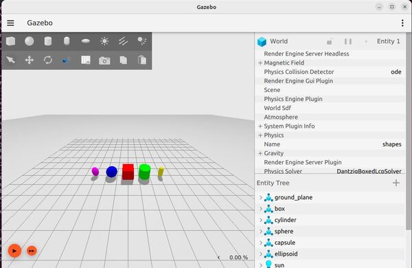
• Start Gazebo
• Spawn the robot
• Start the robot_state_publisher
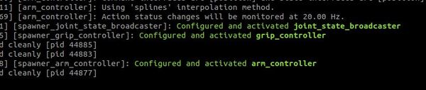
• Load and start the necessary controllers (joint_state_broadcaster, arm_controller, grip_controller)

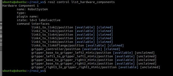
If you look in the logs, you will see the joint_state_broadcaster, arm_controller, and grip_controller are loaded and activated.

Launch MoveIt and RViz.

ros2 launch mycobot_moveit_config_manual_setup move_group.launch.py 

This will:

• Start the move_group node
• Launch RViz with MoveIt configuration
• Use the simulation time from Gazebo

Rather than launching two launch files one after the other, you can put them both into a bash script like this (call the file some name like “robot.sh”):

#!/bin/bash
# Single script to launch the mycobot with Gazebo, RViz, and MoveIt 2

cleanup() {
    echo "Restarting ROS 2 daemon to cleanup before shutting down all processes..."
    ros2 daemon stop
    sleep 1
    ros2 daemon start
    echo "Terminating all ROS 2-related processes..."
    kill 0
    exit
}

trap 'cleanup' SIGINT;
ros2 launch mycobot_gazebo mycobot_280_arduino_bringup_ros2_control_gazebo.launch.py use_rviz:=false &
sleep 10
ros2 launch mycobot_moveit_config_manual_setup move_group.launch.py

Be sure to set permissions to this bash script before running it.

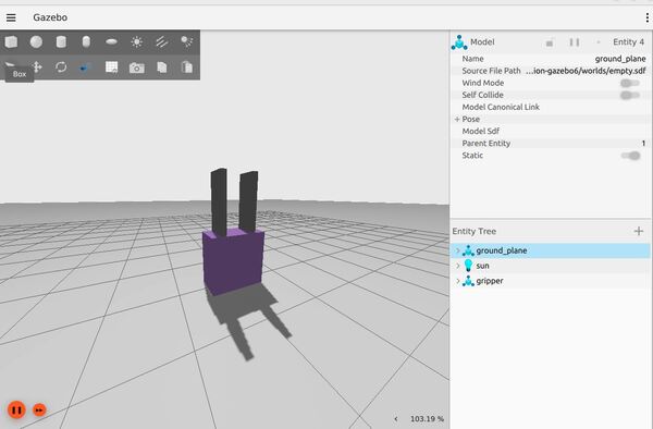
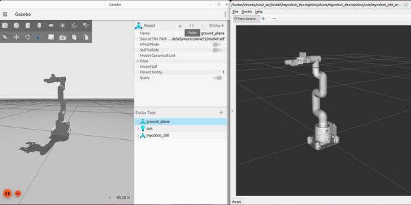
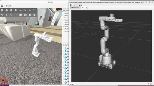
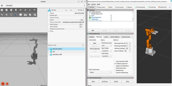
sudo chmod +x robot.sh

Then run this command to launch everything at once.

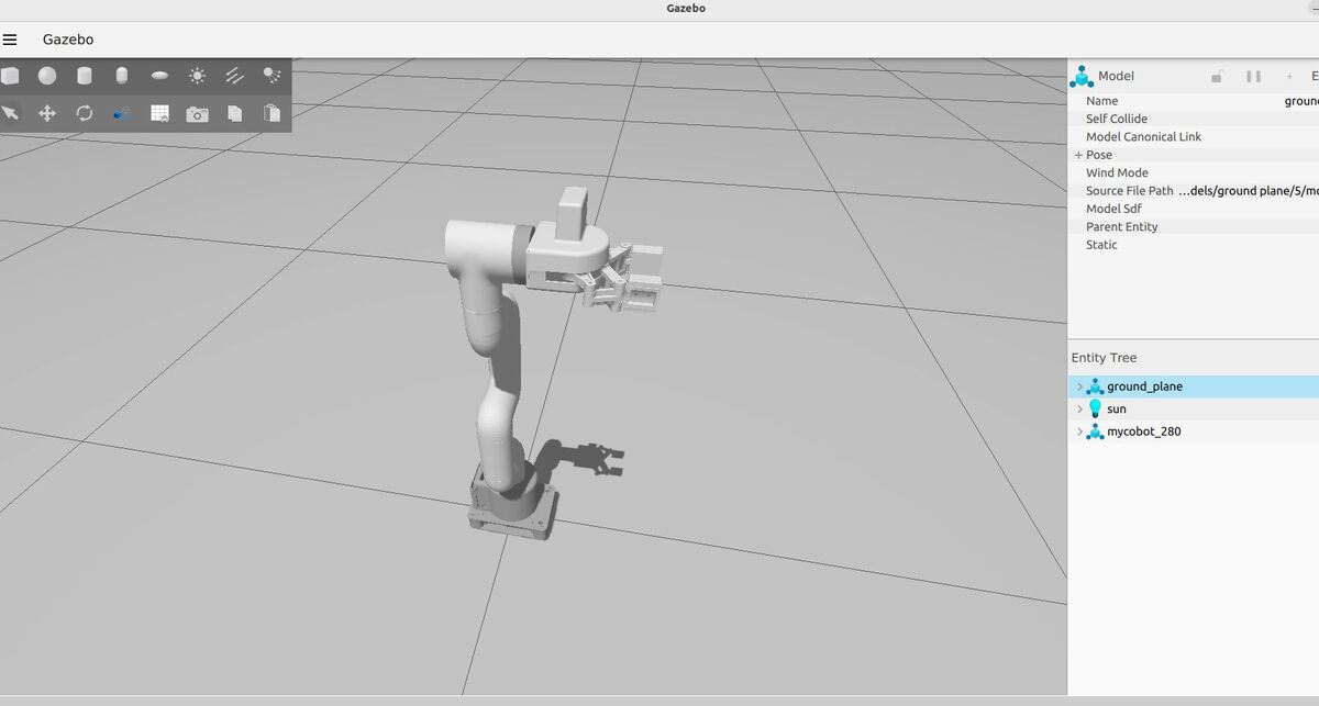
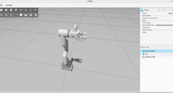
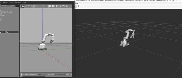
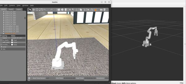
bash robot.sh

Here is what your screen should look like when everything is loaded properly. You will notice that on the right-hand side of Gazebo I closed the two panels. You can close them by right-clicking and hitting “Close”.

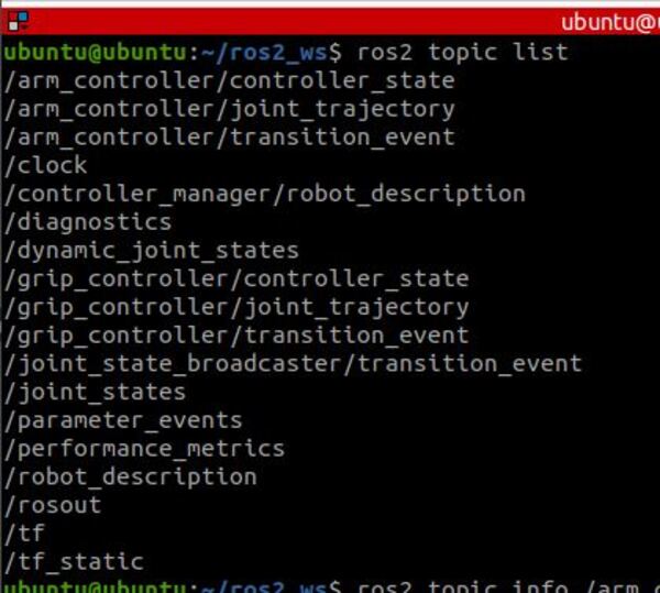
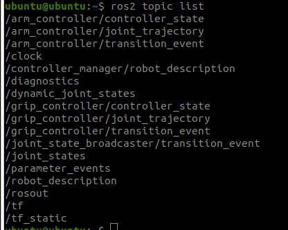
Let’s check out the active topics:

ros2 topic list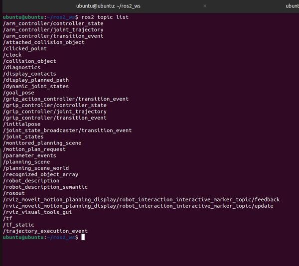

The active nodes are:

ros2 node list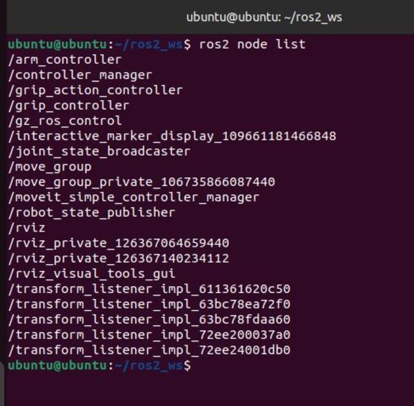

Here are our available action servers:

ros2 action list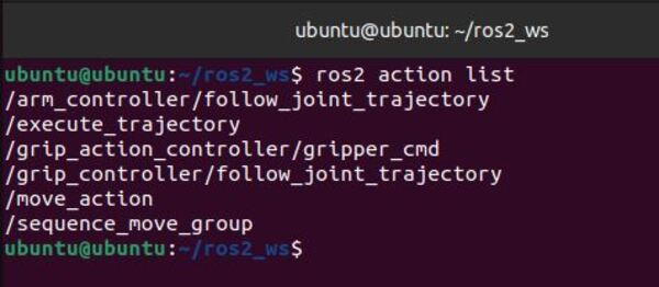

Here are our services. You will see we have a lot of services. This page at the ROS 2 tutorials shows you how we can call services from the command line.

ros2 service list

Let’s check out the parameters for the different nodes my launching a GUI tool called rqt_reconfigure:

sudo apt install ros-$ROS_DISTRO-rqt-reconfigure

rqt --standalone rqt_reconfigure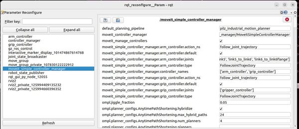

Click “Refresh”.

Click on any of the nodes to see the parameters for that node. For example, let’s take a look at the moveit_simple_controller_manager node.

This tool enables you to see if the parameters you set in the config file of your MoveIt package were set correctly. 

Explore MoveIt in RViz

We will now roughly follow this official MoveIt Quickstart in RViz tutorial which walks you through the main features provided by the MoveIt RViz plugins.

First, click on the Displays panel in the upper left.

Under Global Options, make sure the Fixed Frame is set to “base_link”

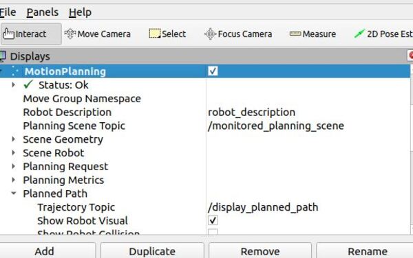
Scroll down to the MotionPlanning plugin.

Make sure the Robot Description field is set to robot_description.

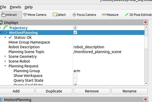
Make sure the Planning Scene Topic field is set to /monitored_planning_scene. 

Make sure the Trajectory Topic under Planned Path is set to /display_planned_path.

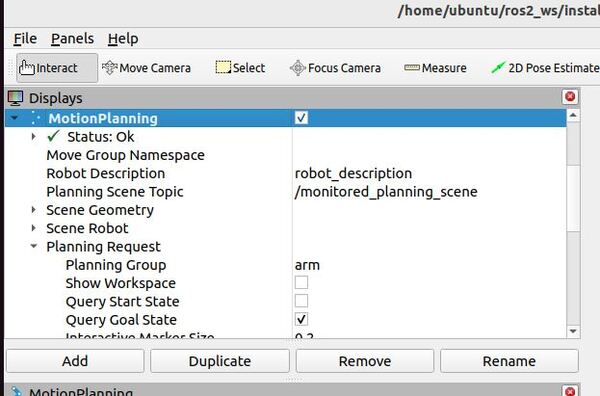
In the Planning Request section,  make sure the Planning Group is set to arm. You can also see this in the MotionPlanning panel in the bottom left.

Play With the Robotic Arm

Rviz has four different visualizations for MoveIt. These visualizations are overlapping.

1. The robot’s configuration in the /monitored_planning_scene planning environment:
   • Planning Scene -> Scene Robot -> Show Robot Visual checkbox
2. The planned path for the robot:
   • Motion Planning -> Planned Path -> Show Robot Visual checkbox
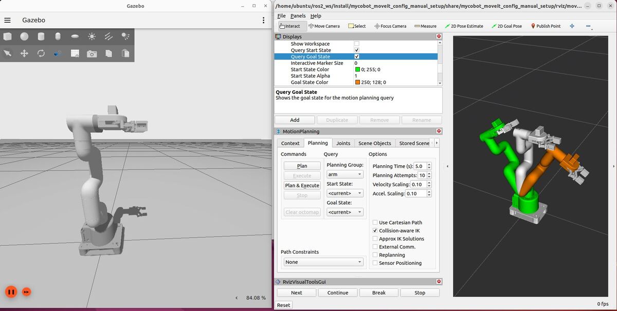
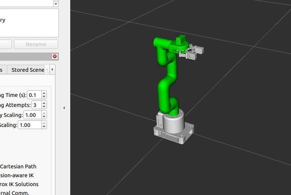
3. Green: The start state for motion planning:
   • MotionPlanning -> Planning Request -> Query Start State checkbox
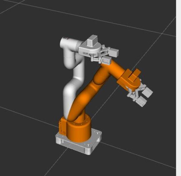
4. Orange: The goal state for motion planning:
   • MotionPlanning -> Planning Request -> Query Goal State checkbox

You can toggle each of these visualizations on and off using the checkboxes in the Displays panel.

Interact With the Robotic Arm

Now let’s configure our RViz so that all we have are the scene robot, the starting state, and the goal state.

1. Check the Motion Planning -> Planned Path -> Show Robot Visual checkbox
2. Uncheck the Planning Scene -> Scene Robot -> Show Robot Visual checkbox
3. Uncheck the MotionPlanning -> Planning Request -> Query Start State checkbox
4. Check the MotionPlanning -> Planning Request -> Query Goal State checkbox

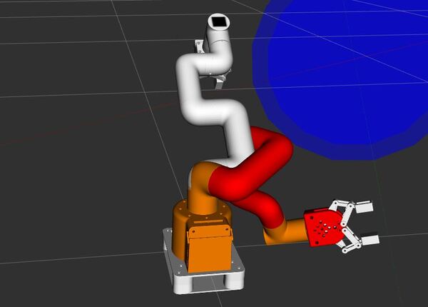
The orange colored robot represents the desired Goal State. 

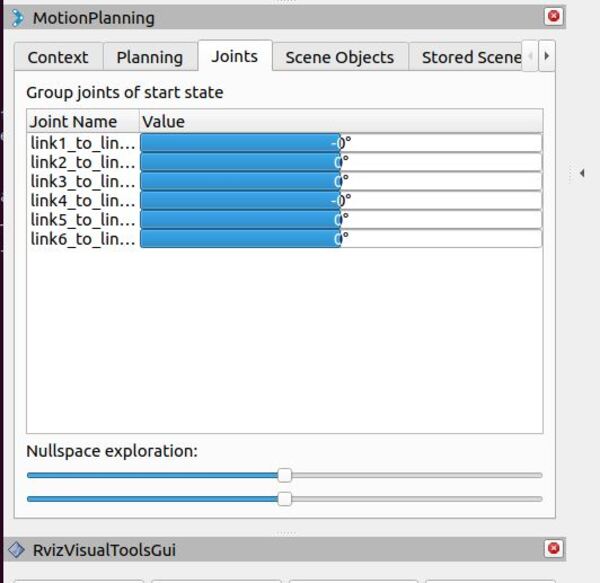
Find the “Joints” tab in the bottom MotionPlanning panel. This lets you control individual joints of the robot.

Try moving the sliders for the joints, and watch how the robot arm changes its pose. 

Uncheck the MotionPlanning -> Planning Request -> Query Goal State checkbox.

Check the MotionPlanning -> Planning Request -> Query Start State checkbox.

The green colored robot is used to set the Start State for motion planning.

Use Motion Planning

Now it’s time to plan a movement for your robotic arm using RViz and MoveIt 2.

In the Displays panel in RViz, do the following…

Uncheck the MotionPlanning -> Planning Request -> Query Goal State checkbox

Check the MotionPlanning -> Planning Request -> Query Start State checkbox.

You can see if any links are in collision by going to the MotionPlanning window at the bottom and moving to the “Status” tab.

Move the green (Start State) to where you want the movement to begin.

Rather than using the interactive marker, I find it easier to go to the “Joints” tab in the Motion Planning window at the bottom. This lets you control individual joints of the robot to get your desired Start State.

Uncheck the MotionPlanning -> Planning Request -> Query Start State checkbox.

Check the MotionPlanning -> Planning Request -> Query Goal State checkbox.

Move the orange (Goal State) to where you want the movement to end.

Check the MotionPlanning -> Planning Request -> Query Start State checkbox.

If you have a strong computer, you can check the MotionPlanning -> Planned Path -> Show Trail checkbox. This will show you a trail of the planned path. This step is optional.

Now let’s plan a motion. Look for the “MotionPlanning” window at the bottom-left part of the screen.

Click the Context tab.

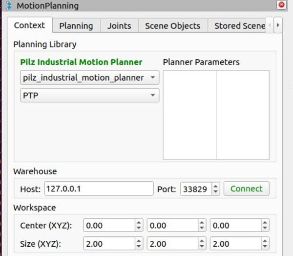
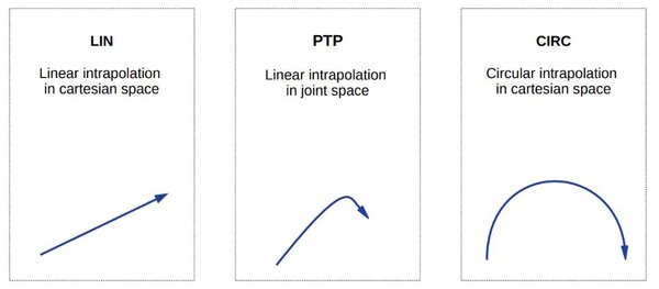
• Select CIRC (circular motion) if you want the end-effector to move in a circular arc.
• Select LIN (linear motion) if you want the end effector to move in a straight line between the start and goal positions
• Select PTP (point-to-point motion) if you want the quickest joint movement between start and goal configurations.

I will click PTP.

Now click the Planning tab.

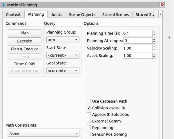
Click the Plan button to generate a motion plan between the start and goal state.

The system will calculate a path, and you should see a preview of the planned motion in the 3D visualization window.

Review the planned path carefully to ensure it’s appropriate and collision-free.

If you’re not satisfied with the plan, you can adjust the start and goal states in the 3D view and plan again.

Once you’re happy with the plan, click the Plan & Execute button to make the robot carry out the planned motion.

You should see your simulated robotic arm moving in both Gazebo and RViz.

If you want to speed things up, you can tweak the Velocity Scaling figures on the Planning tab. You can make them all 1.0 for example.

Then click Plan & Execute again.

Keep setting new Goal States and moving your arm to different poses. 

Be careful not to move your robot into a Goal State where the robot appears red. Red links on your robot mean the robot is colliding with itself.

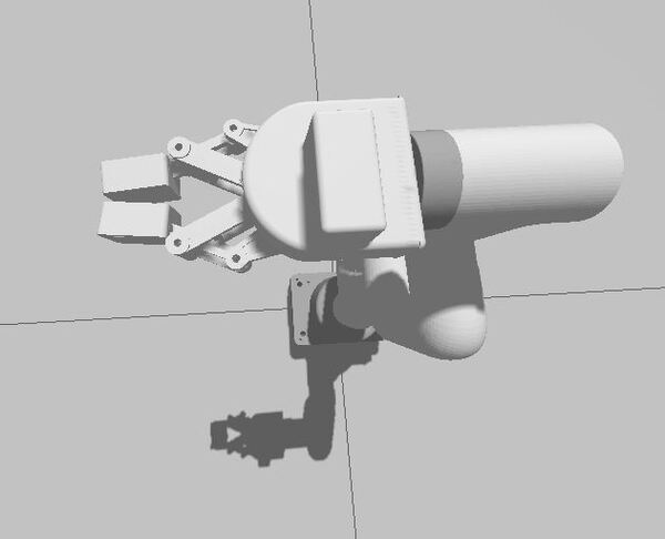
If you want to open and close the gripper. The steps are the same.

Go to the MotionPlanning window at the bottom-left.

Go to the Planning tab.

Change the Planning Group to gripper.

Go to the Context tab.

Select PTP under the pilz_industrial_motion_planner.

Click the Planning tab again.

Select closed as the Goal State. Remember this is one of the states we configured in the SRDF file.

Click Plan & Execute. No need to click Plan first and then Execute since this is a simple motion.

You should see the gripper close in Gazebo.

You can also make motion plans for the combined arm and gripper group. Have fun with it, and play around to get a feel for MoveIt2 in Rviz. 

Don’t forget that every time you change a planning group, you need to go to the Context tab and select PTP.

You can try other planners other than Pilz if you like. 

I have set up OMPL and STOMP as some alternative motion planning libraries. Just use the dropdown menu on the Context tab.

The two parameters files that are required to use OMPL (ompl_planning.yaml) and STOMP (stomp_planning.yaml) are in the mycobot_moveit_config_manual_setup/config folder.

A good planner to use if you are in doubt of what to use is the ompl/RRTConnectkConfigDefault planner. It works well for a wide variety of use cases.

Introspecting Trajectory Waypoints

Understanding how your robot moves in detail is important for ensuring smooth and safe operations. Let’s explore a tool that allows us to do just that:

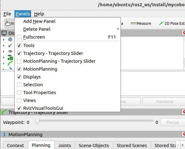
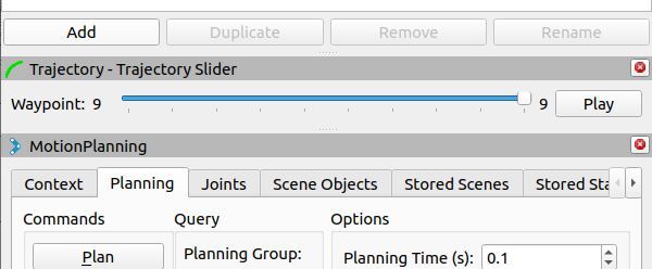
Add a new tool to RViz.

• Click on the “Panels” menu
• Choose “Trajectory – Trajectory Slider”
• You’ll see a new slider appear in RViz

Plan a movement:

• Set a new goal pose for the robotic arm.
• Click the “Plan” button

Use the new Trajectory Slider:

• Move the slider to see each step of the robot’s planned movement
• Press the “Play” button to watch the whole movement smoothly

Remember: If you change where you want the robot to go, always click “Plan” again before using the slider or “Play” button. This makes sure you’re looking at the newest plan, not an old one.

This tool helps you understand exactly how your robot will move from start to finish.

Plan Cartesian Motions

Sometimes, you want your robot to move in a straight line. Here’s how to do that.

Go to the MotionPlanning panel at the bottom-right of the screen.

Click the Planning tab.

Click the Use Cartesian Path checkbox.

What does this do?

• When checked, the robot will try to move its end-effector in a straight line.
• This is useful for tasks that need precise, direct movements, like drawing a straight line or moving directly towards an object.

Why is this important?

• Normal planning might move the robot’s arm in a curved or complex path.
• Cartesian planning ensures a more predictable, straight-line movement.

Try planning some movements with this option on and off to see the difference in how the robot moves.

That’s it! Keep building!

In this tutorial, I will show you how to set up and control a robotic arm using ROS 2 Control and Gazebo (the classic version and the newer version).

By the end of this tutorial, you will be able to create this:

ROS 2 Control is a framework for robots that lets you create programs to control their movement. Think of it as a middleman between the robot hardware and the robot software.

ROS 2 Control connects directly to your hardware (e.g. Arduino) to send commands to the hardware from the software and to receive joint states from the hardware (i.e. the current angular position in radians of each motor of the robotic arm) and send that information out to the rest of ROS 2.

A complete block diagram showing an overview of ROS 2 Control is on this page.

If you look at that block diagram, you will see that the two main building blocks for ROS 2 Control are:

• Controller Manager (managers the controllers, which calculate the commands needed to make the robot behave as desired)
• Resource Manager (manages the hardware interfaces, or communication with the actual robot hardware)

The Controller Manager is responsible for loading, unloading, and managing multiple controllers within the ROS 2 Control framework. It handles the lifecycle of controllers, coordinates their execution, and ensures proper switching between different control modes.

ROS 2 has many different controllers, with some of the most popular being:

1. Joint Position Controller: Inputs a desired joint position and outputs position commands to the hardware.
2. Joint Trajectory Controller: Accepts a trajectory of joint positions over time, from a software like MoveIt2, as input (think of it as a list of goal positions for your robotic arm) and outputs a series of position, velocity, or effort commands to the hardware interface so that arm can follow that trajectory.
3. Diff Drive Controller: Takes velocity commands (linear and angular) from a software such as Nav2 as input and outputs wheel velocities or positions for differential drive robots.

These controllers process their respective inputs to generate appropriate outputs, enabling precise control of various robotic systems from manipulators to mobile platforms.

The Resource Manager manages the hardware resources of the robot (i.e. “Hardware Interface”), providing an abstraction layer between the controllers and the actual hardware. It handles the communication with the physical devices (such as the Arduino on the robotic arm), manages state information (e.g. the current angle of each joint of the robotic arm), and provides a unified interface for controllers to interact with various hardware components.

Prerequisites

• You understand what a joint and link are.
• You have created a ROS 2 workspace.
• You know what a ROS 2 package is.
• You have created a URDF file for a simulated robotic arm that you want to use in Gazebo. I will be using the myCobot 280 for Arduino by Elephant Robotics.
• If you are using a virtual machine on Ubuntu, I recommend you use Oracle VirtualBox instead of VMWare. I had a lot of issues on VMWare that prevented me from running Gazebo.
• I am using ROS 2 Iron, the most recent version at the time of writing this tutorial, but you are welcome to use other versions of ROS 2 if you prefer.
• You have completed my tutorial, “How to Simulate a Robotic Arm in Gazebo – ROS 2”.

All my code for this project is located here on GitHub.

Here is the official documentation for ROS 2 control.

Gazebo (classic version)

Install ROS 2 Control 

To begin, open a terminal window, and install the ROS 2 Control packages (the packages might already be installed):

sudo apt-get install ros-${ROS_DISTRO}-ros2-control ros-${ROS_DISTRO}-ros2-controllers ros-${ROS_DISTRO}-gripper-controllers ros-${ROS_DISTRO}-gazebo-ros2-control

Create the XACRO/URDF Files

Let’s begin by creating some URDF files. Open a new terminal window, and type:

cd ~/ros2_ws/src/mycobot_ros2/mycobot_gazebo/urdf

mkdir -p ros2_control/classic_gazebo

cd ros2_control/classic_gazebo

gedit mycobot_280.urdf.xacro

Add this code. Then save and close.

If you take a look at the file, you will see we have added a <transmissions> element.

The purpose of the <transmission> element is to define how the joint commands from the controllers are mapped to the actual joint motions of the robot.

Historically, in ROS 1, the <transmission> element was commonly used to specify the relationship between the joint commands and the actuator commands. It provided a way to define the gearing ratio, mechanical reduction, and other properties related to the transmission of motion from the actuators to the joints.

In general, when using the ros2_control framework in ROS 2, the <transmission> element is not strictly necessary in the XACRO files. The joint-actuator mapping and control-related configurations are typically handled through the controller configuration YAML files and the hardware interface layer.

gedit mycobot_280_classic_gazebo.xacro

Add this code. Then save and close.

This XML code defines a Gazebo plugin for a robot named “mycobot_280” using the ROS 2 control framework. It specifies the robot description, robot state publisher node, and the location of the controller configuration YAML file for the mycobot_280 robot.

gedit mycobot_280_ros2_control.xacro

Add this code. Then save and close.

This XML code defines the interface between the robot’s hardware and the ROS 2 Control library for a robot named “mycobot_280”. It specifies the joint names, their command and state interfaces, and the minimum and maximum position limits for each joint, including the gripper joints with mimic properties.

If you take a closer look at the file, you can see that ROS 2 Control provides a structured way to handle the hardware interface for different types of robots through a set of standardized components. These components are primarily divided into command interfaces and state interfaces. Here’s an overview of each:

Command Interfaces (write to hardware)

Command interfaces are used for sending commands to hardware components. These commands could be setpoints, desired positions, velocities, or efforts (torque/force) that the hardware should attempt to achieve. Command interfaces are important for motors and are defined based on the type of control you need to exert on a hardware component. Typical command interfaces include:

• Position Commands: Used to set a desired position for the motors.
• Velocity Commands: Used to set a desired velocity for the motors.
• Effort Commands: Used to control motors based on force or torque (e.g. the force to be applied to grasp an object)

These interfaces allow controllers to interact directly with the hardware abstraction layers, issuing commands that the hardware then tries to follow based on its capabilities and feedback mechanisms.

State Interfaces (read from hardware)

State interfaces are used to read the current state of the hardware components. These are essential for monitoring and feedback loops in control systems. State interfaces provide real-time data on various parameters such as position, velocity, effort, and other specific sensor readings. Common types of state interfaces include:

• Position State: Provides the current position of actuators or sensors.
• Velocity State: Gives the current velocity of moving parts.
• Effort State: Indicates the current force or torque being applied by actuators.

In practice, to use ros2_control, you define these interfaces in a YAML configuration file (see next section) where you specify each joint or hardware component along with its corresponding command and state interfaces. This configuration is then loaded and managed by a controller manager, which handles the life cycle and updates of each controller in real-time.

This framework allows developers to focus more on the higher-level control strategies rather than the specifics of each hardware component, promoting reusability and scalability in robotics applications.

Create a YAML Configuration File for the Controller Manager

In this section, we will create a YAML configuration file that defines the controllers and their properties for our robotic arm. The controller manager in ROS 2 Control uses this file to load and configure the appropriate controllers during runtime.

The YAML file allows us to specify the joint controllers, their types, and associated parameters. By creating a well-structured configuration file, we can easily manage and control the behavior of our robotic arm in the Gazebo simulation environment.

We will walk through the process of creating the YAML file step by step, explaining each part and its significance. By the end of this section, you will have a complete configuration file ready to be used with the controller manager in your ROS 2 Control setup.

cd ~/ros2_ws/src/mycobot_ros2/mycobot_gazebo/config

gedit mycobot_280_controllers.yaml

Add this code, and save it.

# controller_manager provides the necessary infrastructure to manage multiple controllers efficiently and robustly.
controller_manager:
  ros__parameters:
    update_rate: 10 # update_rate specifies how often (in Hz) the controllers should be updated.

    # The JointTrajectoryController allows you to send joint trajectory commands to a group 
    # of joints on a robot. These commands specify the desired positions for each joint.     
    arm_controller:
      type: joint_trajectory_controller/JointTrajectoryController

    grip_controller:
      type: joint_trajectory_controller/JointTrajectoryController

    # Responsible for publishing the current state of the robot's joints to the /joint_states 
    # ROS 2 topic
    joint_state_broadcaster:
      type: joint_state_broadcaster/JointStateBroadcaster

# Define the parameters for each controller
arm_controller:
  ros__parameters:
    joints:
      - link1_to_link2
      - link2_to_link3
      - link3_to_link4
      - link4_to_link5
      - link5_to_link6
      - link6_to_link6flange

    # The controller will expect position commands as input for each of these joints.
    command_interfaces:
      - position
    
    # Tells the controller that it should expect to receive position data as the state 
    # feedback from the hardware interface,
    state_interfaces:
      - position

    # If true, When set to true, the controller will not use any feedback from the system 
    # (e.g., joint positions, velocities, efforts) to compute the control commands. 
    open_loop_control: true

    # When set to true, it allows the controller to integrate the trajectory goals it receives. 
    # This means that if the goal trajectory only specifies positions, the controller will 
    # numerically integrate the positions to compute the velocities and accelerations required 
    # to follow the trajectory.
    allow_integration_in_goal_trajectories: true

grip_controller:
  ros__parameters:
    joints:
      - gripper_controller
      
    command_interfaces:
      - position

    state_interfaces:
      - position

    open_loop_control: true
    allow_integration_in_goal_trajectories: true

Here’s a brief explanation of the different parts of the YAML file:

1. controller_manager: This section defines the configuration for the controller manager, which is responsible for managing multiple controllers in the system.

2. arm_controller and grip_controller: These sections define the configuration for the arm and grip controllers, respectively. Both controllers are of type joint_trajectory_controller/JointTrajectoryController, which allows sending joint trajectory commands to a group of joints.

3. joint_state_broadcaster: This section defines the configuration for the joint state broadcaster, which is responsible for publishing the current state of the robot’s joints to the /joint_states ROS 2 topic. It is of type joint_state_broadcaster/JointStateBroadcaster.

4. ros__parameters under each controller:

• joints: Specifies the list of joints that the controller should control. In this case, the arm controller controls joints from `link1_to_link2` to `link6_to_link6flange`, while the grip controller controls the `gripper_controller` joint.
• command_interfaces: Specifies the type of command interface the controller expects. In this case, both controllers expect position commands.
• state_interfaces: Specifies the type of state feedback the controller expects from the hardware interface. Here, both controllers expect position feedback.
• open_loop_control: When set to true, the controller will not use any feedback from the system (e.g., joint positions, velocities, efforts) to compute the control commands. It will solely rely on the provided commands.
• allow_integration_in_goal_trajectories: When set to true, the controller will integrate the trajectory goals it receives. If the goal trajectory only specifies positions, the controller will numerically integrate the positions to compute the velocities and accelerations required to follow the trajectory.

Create a Launch File

cd ~/ros2_ws/src/mycobot_ros2/mycobot_gazebo/launch

gedit mycobot_280_arduino_bringup_ros2_control_classic_gazebo.launch.py

Add this code, and save.

Now build the package.

cd ~/ros2_ws/

colcon build

source ~/.bashrc

Launch Everything and Move the Arm

Now launch everything:

ros2 launch mycobot_gazebo mycobot_280_arduino_bringup_ros2_control_classic_gazebo.launch.py

See the active controllers:

ros2 control list_controllers

To get more information, type:

ros2 control list_controllers -v

To see a list of all the commands you can use type:

ros2 control 

Then press Tab twice.

List all the available hardware components that are loaded and ready to be used by the ros2_control controller manager.

ros2 control list_hardware_components

Now let’s send a command to the robotic arm to move it.

Let’s check out the topics:

ros2 topic list

We need this topic: /arm_controller/joint_trajectory

We can publish a trajectory to that topic to move the arm. Let’s get more information about the topic:

ros2 topic info /arm_controller/joint_trajectory

We need we need to publish a message of type:

trajectory_msgs/msg/JointTrajectory

Remember, here were the list of joints that are controlled by the arm_controller:

• link1_to_link2
• link2_to_link3
• link3_to_link4
• link4_to_link5
• link5_to_link6
• link6_to_link6flange

There are 6 joints in total.

Here is a command you can try:

ros2 topic pub --once /arm_controller/joint_trajectory trajectory_msgs/msg/JointTrajectory "{joint_names: ['link1_to_link2', 'link2_to_link3', 'link3_to_link4', 'link4_to_link5', 'link5_to_link6', 'link6_to_link6flange'], points: [{positions: [-1.345, -1.23, 0.264, -0.296, 0.389, -1.5], time_from_start: {sec: 5, nanosec: 0}}]}"

You can also move it back home now:

ros2 topic pub --once /arm_controller/joint_trajectory trajectory_msgs/msg/JointTrajectory "{joint_names: ['link1_to_link2', 'link2_to_link3', 'link3_to_link4', 'link4_to_link5', 'link5_to_link6', 'link6_to_link6flange'], points: [{positions: [0.0, 0.0, 0.0, 0.0, 0.0, 0.0], time_from_start: {sec: 5, nanosec: 0}}]}"

To close the gripper, you can type:

ros2 topic pub /grip_controller/joint_trajectory trajectory_msgs/msg/JointTrajectory "{joint_names: ['gripper_controller'], points: [{positions: [-0.70], time_from_start: {sec: 5} } ]}" --once

To open the gripper, you can type:

ros2 topic pub /grip_controller/joint_trajectory trajectory_msgs/msg/JointTrajectory "{joint_names: ['gripper_controller'], points: [{positions: [0.0], time_from_start: {sec: 5} } ]}" --once

That’s it for Gazebo Classic.

Gazebo (new version – recommended)

Now let’s run through the process for ROS 2 Control using the newer version of Gazebo. 

Install ROS 2 Control

Open a new terminal window, and type

sudo apt update

sudo apt install ros-${ROS_DISTRO}-gz-ros2-control

Check your installation:

ros2 pkg list | grep gz_ros2_control

You can also install the gz_ros2_control_demos package.

sudo apt install ros-${ROS_DISTRO}-gz-ros2-control-demos

To run the gripper example, type:

ros2 launch gz_ros2_control_demos gripper_mimic_joint_example.launch.py

To move the gripper, type:

ros2 run gz_ros2_control_demos example_gripper

You can try the differential drive mobile robot example as well:

ros2 launch gz_ros2_control_demos diff_drive_example.launch.py

To move the robot, type:

ros2 run gz_ros2_control_demos example_diff_drive 

Create the XACRO/URDF Files

Open a new terminal window, and type:

cd ~/ros2_ws/src/mycobot_ros2/mycobot_gazebo/urdf/ros2_control

mkdir gazebo

cd gazebo

gedit mycobot_280.urdf.xacro

Add this code. Then save and close.

gedit mycobot_280_gazebo.xacro

Take a look at the file. The main body of the robot consists of a base and six arm segments. These segments are joined together in a way that allows them to rotate, much like your own arm can rotate at different points. At the end of the arm, there’s a part called a flange, which is where the gripper is attached.

The gripper has several small parts that work together to allow it to open and close, mimicking the action of fingers grasping an object. T

For each part of the robot, the file describes both how it looks (its “visual” properties) and its physical shape for the purpose of detecting collisions with other objects. Many of these descriptions use 3D mesh files to define complex shapes accurately.

The file also includes information about the physical properties of each part, such as its mass and how that mass is distributed. This is important for simulating how the robot would move and interact with objects in the real world.

The joints that allow the robot’s parts to move have defined limits on how far and how fast they can rotate. This ensures that the simulated robot behaves like its real-world counterpart, preventing unrealistic movements.

Finally, the file includes some information about how the robot should appear in the Gazebo simulation environment, specifying colors and materials for different parts.

Now let’s create some more code. This file is one of the files that we imported in the URDF file we just created. Open a terminal window, and type this:

gedit mycobot_280_gazebo.xacro

Add this code below. Then save and close.

<?xml version="1.0" ?>
<robot xmlns:xacro="http://wiki.ros.org/xacro" name="mycobot_280">
    <gazebo>
        <plugin filename="gz_ros2_control-system" name="gz_ros2_control::GazeboSimROS2ControlPlugin">
            <parameters>$(find mycobot_gazebo)/config/mycobot_280_controllers.yaml</parameters>
            <ros>                <remapping>/controller_manager/robot_description:=/robot_description</remapping>
            </ros>
        </plugin>
    </gazebo>
</robot>

The GazeboSimROS2ControlPlugin is a bridge between the Gazebo simulation environment and ROS 2 control systems. It does the following:

• Loads and initializes the ROS 2 controller manager.
• Sets up the simulation environment
• Manages the overall integration between Gazebo and ROS 2 control

Pay careful attention to the remapping of the topics. The controller manager subscribes to the URDF via the /controller_manager/robot_description topic by default. You need to remap this subscription to the /robot_description topic, which is published by the robot state publisher.

You can learn more about this plugin here on GitHub.

Remember from our last tutorial that the ROS 2 controller manager manages the controllers, like the Joint Trajectory Controller or the Differential Drive Controller.

The Joint Trajectory Controller takes as input trajectory_msgs/msg/JointTrajectory messages from a software like MoveIt2 and outputs commands to the hardware interface (which is managed by the Resource Manager.

You can find a complete list of controllers on this page.

Let’s continue. Open a terminal window, and type:

gedit mycobot_280_ros2_control.xacro

Add this code below. Then save and close.

<?xml version="1.0" ?>

<robot xmlns:xacro="http://wiki.ros.org/xacro" name="mycobot_280">
    <ros2_control name="RobotSystem" type="system">
        <hardware>
            <plugin>gz_ros2_control/GazeboSimSystem</plugin>
        </hardware>

        <joint name="link1_to_link2">
            <command_interface name="position">
                <param name="min">-2.879793</param>
                <param name="max">2.879793</param>
            </command_interface>
            <state_interface name="position"/>
        </joint>

        <joint name="link2_to_link3">
            <command_interface name="position">
                <param name="min">-2.879793</param>
                <param name="max">2.879793</param>
            </command_interface>
            <state_interface name="position"/>
        </joint>

        <joint name="link3_to_link4">
            <command_interface name="position">
                <param name="min">-2.879793</param>
                <param name="max">2.879793</param>
            </command_interface>
            <state_interface name="position"/>
        </joint>

        <joint name="link4_to_link5">
            <command_interface name="position">
                <param name="min">-2.879793</param>
                <param name="max">2.879793</param>
            </command_interface>
            <state_interface name="position"/>
        </joint>

        <joint name="link5_to_link6">
            <command_interface name="position">
                <param name="min">-2.879793</param>
                <param name="max">2.879793</param>
            </command_interface>
            <state_interface name="position"/>
        </joint>

        <joint name="link6_to_link6flange">
            <command_interface name="position">
                <param name="min">-3.05</param>
                <param name="max">3.05</param>
            </command_interface>
            <state_interface name="position"/>
        </joint>

        <joint name="gripper_controller">
            <command_interface name="position">
                <param name="min">-0.7</param>
                <param name="max">0.15</param>
            </command_interface>
            <state_interface name="position"/>
            <state_interface name="velocity"/> 
        </joint>

        <joint name="gripper_base_to_gripper_left2">
            <param name="mimic">gripper_controller</param>
            <param name="multiplier">1.0</param>
            <command_interface name="position">
                <param name="min">-0.8</param>
                <param name="max">0.5</param>
            </command_interface>
            <state_interface name="position"/>
            <state_interface name="velocity"/> 
        </joint>

        <joint name="gripper_left3_to_gripper_left1">
            <param name="mimic">gripper_controller</param>
            <param name="multiplier">-1.0</param>
            <command_interface name="position">
                <param name="min">-0.5</param>
                <param name="max">0.5</param>
            </command_interface>
            <state_interface name="position"/>
            <state_interface name="velocity"/> 
        </joint>

        <joint name="gripper_base_to_gripper_right3">
            <param name="mimic">gripper_controller</param>
            <param name="multiplier">-1.0</param>
            <command_interface name="position">
                <param name="min">-0.15</param>
                <param name="max">0.7</param>
            </command_interface>
            <state_interface name="position"/>
            <state_interface name="velocity"/> 
        </joint>

        <joint name="gripper_base_to_gripper_right2">
            <param name="mimic">gripper_controller</param>
            <param name="multiplier">-1.0</param>
            <command_interface name="position">
                <param name="min">-0.5</param>
               <param name="max">0.8</param>
            </command_interface>
            <state_interface name="position"/>
            <state_interface name="velocity"/> 
        </joint>

        <joint name="gripper_right3_to_gripper_right1">
            <param name="mimic">gripper_controller</param>
            <param name="multiplier">1.0</param>
            <command_interface name="position">
                <param name="min">-0.5</param>
                <param name="max">0.5</param>
            </command_interface>
            <state_interface name="position"/>
            <state_interface name="velocity"/> 
        </joint>
    </ros2_control>    
</robot>

The GazeboSimSystem plugin does the following:

• Implements the specific hardware interfaces for joints and sensors
• Handles the direct read/write operations with the simulated hardware

GazeboSimROS2ControlPlugin loads the Controller Manager, while GazeboSimSystem implements the specific hardware interface that allows ROS 2 controllers (which are managed by the Controller Manager) to send and receive data from the the simulated robotic arm in Gazebo. They work together to provide a complete bridge between Gazebo simulation and ROS 2 control systems.

Create a Launch File

cd ~/ros2_ws/src/mycobot_ros2/mycobot_gazebo/launch

gedit mycobot_280_arduino_bringup_ros2_control_gazebo.launch.py

Add this code below, and save.

# Author: Addison Sears-Collins
# Date: July 30, 2024
# Description: Launch a robotic arm in Gazebo 

import os
from launch import LaunchDescription
from launch.actions import AppendEnvironmentVariable, DeclareLaunchArgument, ExecuteProcess, IncludeLaunchDescription
from launch.actions import RegisterEventHandler
from launch.conditions import IfCondition
from launch.event_handlers import OnProcessExit
from launch.launch_description_sources import PythonLaunchDescriptionSource
from launch.substitutions import LaunchConfiguration
from launch_ros.actions import Node
from launch_ros.substitutions import FindPackageShare
import xacro


def generate_launch_description():

  # Constants for paths to different files and folders
  package_name_description = 'mycobot_description'
  package_name_gazebo = 'mycobot_gazebo'

  default_robot_name = 'mycobot_280'
  gazebo_launch_file_path = 'launch'
  gazebo_models_path = 'models'
  rviz_config_file_path = 'rviz/mycobot_280_arduino_view_description.rviz'
  urdf_file_path = 'urdf/ros2_control/gazebo/mycobot_280.urdf.xacro'
  world_file_path = 'worlds/empty.world' # e.g. 'world/empty.world', 'world/house.world'



  # Set the path to different files and folders.  
  pkg_ros_gz_sim = FindPackageShare(package='ros_gz_sim').find('ros_gz_sim')  
  pkg_share_description = FindPackageShare(package=package_name_description).find(package_name_description)
  pkg_share_gazebo = FindPackageShare(package=package_name_gazebo).find(package_name_gazebo)

  default_rviz_config_path = os.path.join(pkg_share_description, rviz_config_file_path)  
  default_urdf_model_path = os.path.join(pkg_share_gazebo, urdf_file_path)
  gazebo_launch_file_path = os.path.join(pkg_share_gazebo, gazebo_launch_file_path)   
  gazebo_models_path = os.path.join(pkg_share_gazebo, gazebo_models_path)
  world_path = os.path.join(pkg_share_gazebo, world_file_path)

 
  # Launch configuration variables specific to simulation
  robot_name = LaunchConfiguration('robot_name')
  rviz_config_file = LaunchConfiguration('rviz_config_file')
  use_robot_state_pub = LaunchConfiguration('use_robot_state_pub')
  use_rviz = LaunchConfiguration('use_rviz')
  use_sim_time = LaunchConfiguration('use_sim_time')
  world = LaunchConfiguration('world')

  # Set the default pose
  x = LaunchConfiguration('x')
  y = LaunchConfiguration('y')
  z = LaunchConfiguration('z')
  roll = LaunchConfiguration('roll')
  pitch = LaunchConfiguration('pitch')
  yaw = LaunchConfiguration('yaw')

  # Declare the launch arguments  
  declare_robot_name_cmd = DeclareLaunchArgument(
    name='robot_name',
    default_value=default_robot_name,
    description='The name for the robot')

  declare_rviz_config_file_cmd = DeclareLaunchArgument(
    name='rviz_config_file',
    default_value=default_rviz_config_path,
    description='Full path to the RVIZ config file to use')

  declare_use_robot_state_pub_cmd = DeclareLaunchArgument(
    name='use_robot_state_pub',
    default_value='True',
    description='Whether to start the robot state publisher')

  declare_use_rviz_cmd = DeclareLaunchArgument(
    name='use_rviz',
    default_value='True',
    description='Whether to start RVIZ')
    
  declare_use_sim_time_cmd = DeclareLaunchArgument(
    name='use_sim_time',
    default_value='true',
    description='Use simulation (Gazebo) clock if true')

  declare_world_cmd = DeclareLaunchArgument(
    name='world',
    default_value=world_path,
    description='Full path to the world model file to load')

  declare_x_cmd = DeclareLaunchArgument(
    name='x',
    default_value='0.0',
    description='x component of initial position, meters')

  declare_y_cmd = DeclareLaunchArgument(
    name='y',
    default_value='0.0',
    description='y component of initial position, meters')
    
  declare_z_cmd = DeclareLaunchArgument(
    name='z',
    default_value='0.05',
    description='z component of initial position, meters')
    
  declare_roll_cmd = DeclareLaunchArgument(
    name='roll',
    default_value='0.0',
    description='roll angle of initial orientation, radians')

  declare_pitch_cmd = DeclareLaunchArgument(
    name='pitch',
    default_value='0.0',
    description='pitch angle of initial orientation, radians')

  declare_yaw_cmd = DeclareLaunchArgument(
    name='yaw',
    default_value='0.0',
    description='yaw angle of initial orientation, radians')
    
  # Specify the actions

  set_env_vars_resources = AppendEnvironmentVariable(
    'GZ_SIM_RESOURCE_PATH',
    gazebo_models_path)

  # Start arm controller
  start_arm_controller_cmd = ExecuteProcess(
    cmd=['ros2', 'control', 'load_controller', '--set-state', 'active',
        'arm_controller'],
        output='screen')

  # Start Gazebo environment
  start_gazebo_cmd = IncludeLaunchDescription(
    PythonLaunchDescriptionSource(
      os.path.join(pkg_ros_gz_sim, 'launch', 'gz_sim.launch.py')),
    launch_arguments=[('gz_args', [' -r -v 4 ', world])])

  # Start gripper controller
  start_gripper_controller_cmd =  ExecuteProcess(
    cmd=['ros2', 'control', 'load_controller', '--set-state', 'active',
        'grip_controller'],
        output='screen')

  # Start gripper action controller
  start_gripper_action_controller_cmd = ExecuteProcess(
    cmd=['ros2', 'control', 'load_controller', '--set-state', 'active',
        'grip_action_controller'],
        output='screen')
  
  # Launch joint state broadcaster
  start_joint_state_broadcaster_cmd = ExecuteProcess(
    cmd=['ros2', 'control', 'load_controller', '--set-state', 'active',
        'joint_state_broadcaster'],
        output='screen')
    
  # Subscribe to the joint states of the robot, and publish the 3D pose of each link.
  doc = xacro.parse(open(default_urdf_model_path))
  xacro.process_doc(doc)
  start_robot_state_publisher_cmd = Node(
    condition=IfCondition(use_robot_state_pub),
    package='robot_state_publisher',
    executable='robot_state_publisher',
    name='robot_state_publisher',
    output='screen',
    parameters=[{
      'use_sim_time': use_sim_time, 
      'robot_description': doc.toxml()}])

  # Launch RViz
  start_rviz_cmd = Node(
    condition=IfCondition(use_rviz),
    package='rviz2',
    executable='rviz2',
    name='rviz2',
    output='screen',
    arguments=['-d', rviz_config_file],
    parameters=[{'use_sim_time': use_sim_time}])  
    
   
  # Spawn the robot
  start_gazebo_ros_spawner_cmd = Node(
    package='ros_gz_sim',
    executable='create',
    arguments=[
      '-string', doc.toxml(),
      '-name', robot_name,
      '-allow_renaming', 'true',
      '-x', x,
      '-y', y,
      '-z', z,
      '-R', roll,
      '-P', pitch,
      '-Y', yaw
      ],
    output='screen')

  # Launch the joint state broadcaster after spawning the robot
  load_joint_state_broadcaster_cmd = RegisterEventHandler(
     event_handler=OnProcessExit(
     target_action=start_gazebo_ros_spawner_cmd ,
     on_exit=[start_joint_state_broadcaster_cmd],))

  # Launch the arm controller after launching the joint state broadcaster
  load_arm_controller_cmd = RegisterEventHandler(
    event_handler=OnProcessExit(
    target_action=start_joint_state_broadcaster_cmd,
    on_exit=[start_arm_controller_cmd],))

  # Launch the gripper controller after launching the arm controller
  load_gripper_controller_cmd = RegisterEventHandler(
    event_handler=OnProcessExit(
    target_action=start_arm_controller_cmd,
    on_exit=[start_gripper_controller_cmd],))
    
  # Launch the gripper action controller after launching the gripper controller
  load_gripper_action_controller_cmd = RegisterEventHandler(
    event_handler=OnProcessExit(
    target_action=start_gripper_controller_cmd,
    on_exit=[start_gripper_action_controller_cmd],))    

  # Create the launch description and populate
  ld = LaunchDescription()

  # Declare the launch options
  ld.add_action(declare_robot_name_cmd)
  ld.add_action(declare_rviz_config_file_cmd)
  ld.add_action(declare_use_robot_state_pub_cmd)  
  ld.add_action(declare_use_rviz_cmd) 
  ld.add_action(declare_use_sim_time_cmd)
  ld.add_action(declare_world_cmd)

  ld.add_action(declare_x_cmd)
  ld.add_action(declare_y_cmd)
  ld.add_action(declare_z_cmd)
  ld.add_action(declare_roll_cmd)
  ld.add_action(declare_pitch_cmd)
  ld.add_action(declare_yaw_cmd)  

  # Add any actions
  ld.add_action(set_env_vars_resources)
  ld.add_action(start_gazebo_cmd)
  ld.add_action(start_robot_state_publisher_cmd)
  ld.add_action(start_rviz_cmd)
  
  ld.add_action(start_gazebo_ros_spawner_cmd)

  ld.add_action(load_joint_state_broadcaster_cmd)
  ld.add_action(load_arm_controller_cmd) 
  ld.add_action(load_gripper_controller_cmd) 
  ld.add_action(load_gripper_action_controller_cmd)

  return ld

Now build the package.

cd ~/ros2_ws/

colcon build

source ~/.bashrc

Launch Everything and Move the Arm

Now launch everything:

ros2 launch mycobot_gazebo mycobot_280_arduino_bringup_ros2_control_gazebo.launch.py

See the active controllers:

ros2 control list_controllers

To get more information, type:

ros2 control list_controllers -v

If you want to close the gripper, you can do this:

ros2 action send_goal /grip_action_controller/gripper_cmd control_msgs/action/GripperCommand "{command: {position: -0.7, max_effort: 5.0}}"

If you want to open the gripper, you can do this:

ros2 action send_goal /grip_action_controller/gripper_cmd control_msgs/action/GripperCommand "{command: {position: 0.0, max_effort: 5.0}}"

Deactivate the grip_action_controller (which uses the position_controllers/GripperActionController interface…we will use this in a later tutorial)

ros2 control set_controller_state grip_action_controller inactive

Activate the grip_controller (which uses the joint_trajectory_controller/JointTrajectoryController interface)

ros2 control set_controller_state grip_controller active

To see a list of all the commands you can use type:

ros2 control 

Then press Tab twice.

List all the available hardware components that are loaded and ready to be used by the ros2_control controller manager.

ros2 control list_hardware_components

Now let’s send a command to the robotic arm to move it.

Let’s check out the topics:

ros2 topic list

We need this topic: /arm_controller/joint_trajectory

We can publish a trajectory to that topic to move the arm. Let’s get more information about the topic:

ros2 topic info /arm_controller/joint_trajectory

We need we need to publish a message of type:

trajectory_msgs/msg/JointTrajectory

Remember, here were the list of joints that are controlled by the arm_controller:

• link1_to_link2
• link2_to_link3
• link3_to_link4
• link4_to_link5
• link5_to_link6
• link6_to_link6flange

There are 6 joints in total.

Here is a command you can try:

ros2 topic pub --once /arm_controller/joint_trajectory trajectory_msgs/msg/JointTrajectory "{joint_names: ['link1_to_link2', 'link2_to_link3', 'link3_to_link4', 'link4_to_link5', 'link5_to_link6', 'link6_to_link6flange'], points: [{positions: [-1.345, -1.23, 0.264, -0.296, 0.389, -1.5], time_from_start: {sec: 3, nanosec: 0}}]}"

You can also move it back home now:

ros2 topic pub --once /arm_controller/joint_trajectory trajectory_msgs/msg/JointTrajectory "{joint_names: ['link1_to_link2', 'link2_to_link3', 'link3_to_link4', 'link4_to_link5', 'link5_to_link6', 'link6_to_link6flange'], points: [{positions: [0.0, 0.0, 0.0, 0.0, 0.0, 0.0], time_from_start: {sec: 3, nanosec: 0}}]}"

To close the gripper, you can type:

ros2 topic pub /grip_controller/joint_trajectory trajectory_msgs/msg/JointTrajectory "{joint_names: ['gripper_controller'], points: [{positions: [-0.70], time_from_start: {sec: 3.0} } ]}" --once

To open the gripper, you can type:

ros2 topic pub /grip_controller/joint_trajectory trajectory_msgs/msg/JointTrajectory "{joint_names: ['gripper_controller'], points: [{positions: [0.0], time_from_start: {sec: 3.0} } ]}" --once

Move the Robotic Arm Using Code

Let’s create a ROS 2 node that can loop through a list of trajectories to simulate the arm moving from the home position to a goal location and then back to home.

Python

Let’s start by creating a script using Python.

cd ~/ros2_ws/src/mycobot_ros2/mycobot_gazebo/scripts

gedit example_joint_trajectory_publisher.py

Add this code and save the file.

#! /usr/bin/env python3

"""
Description:
  ROS 2: Executes a sample trajectory for a robotic arm in Gazebo
-------
Publishing Topics (ROS 2):
  Desired goal pose of the robotic arm
    /arm_controller/joint_trajectory - trajectory_msgs/JointTrajectory
  
  Desired goal pose of the gripper
    /grip_controller/joint_trajectory - trajectory_msgs/JointTrajectory
-------
Author: Addison Sears-Collins
Date: April 29, 2024
"""

import rclpy # Python client library for ROS 2
from rclpy.node import Node # Handles the creation of nodes
from trajectory_msgs.msg import JointTrajectory, JointTrajectoryPoint
from builtin_interfaces.msg import Duration
from std_msgs.msg import Header  # Import the Header message

# Define constants
arm_joints = [ 'link1_to_link2', 
               'link2_to_link3', 
               'link3_to_link4', 
               'link4_to_link5', 
               'link5_to_link6', 
               'link6_to_link6flange']

gripper_joints = ['gripper_controller']

class ExampleJointTrajectoryPublisherPy(Node):
    """This class executes a sample trajectory for a robotic arm
    
    """      
    def __init__(self):
        """ Constructor.
      
        """
        # Initialize the class using the constructor
        super().__init__('example_joint_trajectory_publisher_py')    
 
        # Create the publisher of the desired arm and gripper goal poses
        self.arm_pose_publisher = self.create_publisher(JointTrajectory, '/arm_controller/joint_trajectory', 1)
        self.gripper_pose_publisher = self.create_publisher(JointTrajectory, '/grip_controller/joint_trajectory', 1)

        self.timer_period = 5.0  # seconds 5.0
        self.timer = self.create_timer(self.timer_period, self.timer_callback)

        self.frame_id = "base_link"
       
        # Desired time from the trajectory start to arrive at the trajectory point.
        # Needs to be less than or equal to the self.timer_period above to allow
        # the robotic arm to smoothly transition between points.
        self.duration_sec = 2 
        self.duration_nanosec = 0.5 * 1e9 # (seconds * 1e9)

        # Set the desired goal poses for the robotic arm.
        self.arm_positions = []
        self.arm_positions.append([0.0, 0.0, 0.0, 0.0, 0.0, 0.0]) # Home location
        self.arm_positions.append([-1.345, -1.23, 0.264, -0.296, 0.389, -1.5]) # Goal location
        self.arm_positions.append([-1.345, -1.23, 0.264, -0.296, 0.389, -1.5]) 
        self.arm_positions.append([0.0, 0.0, 0.0, 0.0, 0.0, 0.0]) # Home location

        self.gripper_positions = []
        self.gripper_positions.append([0.0]) # Open gripper
        self.gripper_positions.append([0.0])
        self.gripper_positions.append([-0.70]) # Close gripper
        self.gripper_positions.append([-0.70]) 

        # Keep track of the current trajectory we are executing
        self.index = 0

    def timer_callback(self):
        """Set the goal pose for the robotic arm.
    
        """
        # Create new JointTrajectory messages
        msg_arm = JointTrajectory()
        msg_arm.header = Header()  
        msg_arm.header.frame_id = self.frame_id  
        msg_arm.joint_names = arm_joints

        msg_gripper = JointTrajectory()
        msg_gripper.header = Header()  
        msg_gripper.header.frame_id = self.frame_id  
        msg_gripper.joint_names = gripper_joints

        # Create JointTrajectoryPoints
        point_arm = JointTrajectoryPoint()
        point_arm.positions = self.arm_positions[self.index]
        point_arm.time_from_start = Duration(sec=int(self.duration_sec), nanosec=int(self.duration_nanosec))  # Time to next position
        msg_arm.points.append(point_arm)
        self.arm_pose_publisher.publish(msg_arm)

        point_gripper = JointTrajectoryPoint()
        point_gripper.positions = self.gripper_positions[self.index]
        point_gripper.time_from_start = Duration(sec=int(self.duration_sec), nanosec=int(self.duration_nanosec))  
        msg_gripper.points.append(point_gripper)
        self.gripper_pose_publisher.publish(msg_gripper)

        # Reset the index
        if self.index == len(self.arm_positions) - 1:
            self.index = 0
        else:
            self.index = self.index + 1
    
def main(args=None):
  
    # Initialize the rclpy library
    rclpy.init(args=args)
  
    # Create the node
    example_joint_trajectory_publisher_py = ExampleJointTrajectoryPublisherPy()
  
    # Spin the node so the callback function is called.
    rclpy.spin(example_joint_trajectory_publisher_py)
    
    # Destroy the node
    example_joint_trajectory_publisher_py.destroy_node()
  
    # Shutdown the ROS client library for Python
    rclpy.shutdown()
  
if __name__ == '__main__':
  main()

Add the code to your CMakeLists.txt file.

cd ~/ros2_ws/

colcon build

source ~/.bashrc

Launch your arm in Gazebo:

ros2 launch mycobot_gazebo mycobot_280_arduino_bringup_ros2_control_gazebo.launch.py

Now run your node:

ros2 run mycobot_gazebo  example_joint_trajectory_publisher.py

C++

Now let’s create the same node in C++.

mkdir ~/ros2_ws/src/mycobot_ros2/mycobot_gazebo/src

mkdir ~/ros2_ws/src/mycobot_ros2/mycobot_gazebo/include

cd src

gedit example_joint_trajectory_publisher.cpp

/**
 * @file example_joint_trajectory_publisher.cpp
 * @brief ROS 2: Executes a sample trajectory for a robotic arm in Gazebo
 * 
 * Publishing Topics (ROS 2):
 *   Desired goal pose of the robotic arm
 *     /arm_controller/joint_trajectory - trajectory_msgs::msg::JointTrajectory
 *   
 *   Desired goal pose of the gripper
 *     /grip_controller/joint_trajectory - trajectory_msgs::msg::JointTrajectory
 * 
 * @author Addison Sears-Collins
 * @date April 29, 2024
 */

#include <chrono>
#include <functional>
#include <memory>
#include <string>

#include "rclcpp/rclcpp.hpp"
#include "trajectory_msgs/msg/joint_trajectory.hpp"
#include "std_msgs/msg/header.hpp"

using namespace std::chrono_literals;

// Define constants
const std::vector<std::string> arm_joints = {
    "link1_to_link2",
    "link2_to_link3",
    "link3_to_link4",
    "link4_to_link5",
    "link5_to_link6",
    "link6_to_link6flange"
};

const std::vector<std::string> gripper_joints = {
    "gripper_controller"
};

class ExampleJointTrajectoryPublisherCpp : public rclcpp::Node
{
public:
    ExampleJointTrajectoryPublisherCpp()
        : Node("example_joint_trajectory_publisher_cpp")
    {
        // Create the publisher of the desired arm and gripper goal poses
        arm_pose_publisher_ = create_publisher<trajectory_msgs::msg::JointTrajectory>("/arm_controller/joint_trajectory", 1);
        gripper_pose_publisher_ = create_publisher<trajectory_msgs::msg::JointTrajectory>("/grip_controller/joint_trajectory", 1);

        // Create a timer to periodically call the timerCallback function
        timer_ = create_wall_timer(5s, std::bind(&ExampleJointTrajectoryPublisherCpp::timerCallback, this));

        frame_id_ = "base_link";

        // Desired time from the trajectory start to arrive at the trajectory point.
        // Needs to be less than or equal to the timer period above to allow
        // the robotic arm to smoothly transition between points.
        duration_sec_ = 2;
        duration_nanosec_ = 0.5 * 1e9;  // (seconds * 1e9)

        // Set the desired goal poses for the robotic arm.
        arm_positions_ = {
            {0.0, 0.0, 0.0, 0.0, 0.0, 0.0},  // Home location
            {-1.345, -1.23, 0.264, -0.296, 0.389, -1.5},  // Goal location
            {-1.345, -1.23, 0.264, -0.296, 0.389, -1.5},
            {0.0, 0.0, 0.0, 0.0, 0.0, 0.0}  // Home location
        };

        gripper_positions_ = {
            {0.0},  // Open gripper
            {0.0},
            {-0.70},  // Close gripper
            {-0.70}
        };

        // Keep track of the current trajectory we are executing
        index_ = 0;
    }

private:
    void timerCallback()
    {
        // Create new JointTrajectory messages for arm and gripper
        auto msg_arm = trajectory_msgs::msg::JointTrajectory();
        msg_arm.header.frame_id = frame_id_;
        msg_arm.joint_names = arm_joints;

        auto msg_gripper = trajectory_msgs::msg::JointTrajectory();
        msg_gripper.header.frame_id = frame_id_;
        msg_gripper.joint_names = gripper_joints;

        // Create JointTrajectoryPoints for arm and gripper
        auto point_arm = trajectory_msgs::msg::JointTrajectoryPoint();
        point_arm.positions = arm_positions_[index_];
        point_arm.time_from_start = rclcpp::Duration(duration_sec_, duration_nanosec_);
        msg_arm.points.push_back(point_arm);
        arm_pose_publisher_->publish(msg_arm);

        auto point_gripper = trajectory_msgs::msg::JointTrajectoryPoint();
        point_gripper.positions = gripper_positions_[index_];
        point_gripper.time_from_start = rclcpp::Duration(duration_sec_, duration_nanosec_);
        msg_gripper.points.push_back(point_gripper);
        gripper_pose_publisher_->publish(msg_gripper);

        // Reset the index 
        if (index_ == arm_positions_.size() - 1) {
            index_ = 0;
        } else {
            index_++;
        }
    }

    // Publishers for arm and gripper joint trajectories
    rclcpp::Publisher<trajectory_msgs::msg::JointTrajectory>::SharedPtr arm_pose_publisher_;
    rclcpp::Publisher<trajectory_msgs::msg::JointTrajectory>::SharedPtr gripper_pose_publisher_;

    // Timer for periodic callback
    rclcpp::TimerBase::SharedPtr timer_;

    // Frame ID for the joint trajectories
    std::string frame_id_;

    // Duration for each trajectory point
    int duration_sec_;
    int duration_nanosec_;

    // Desired goal poses for the robotic arm and gripper
    std::vector<std::vector<double>> arm_positions_;
    std::vector<std::vector<double>> gripper_positions_;

    // Index to keep track of the current trajectory point
    size_t index_;
};

int main(int argc, char * argv[])
{
    // Initialize the ROS 2 client library
    rclcpp::init(argc, argv);

    // Create an instance of the ExampleJointTrajectoryPublisherCpp node
    auto node = std::make_shared<ExampleJointTrajectoryPublisherCpp>();

    // Spin the node to execute the callbacks
    rclcpp::spin(node);

    // Shutdown the ROS 2 client library
    rclcpp::shutdown();

    return 0;
}

Update your CMakeLists.txt file and package.xml file.

cd ~/ros2_ws/

colcon build

source ~/.bashrc

Launch your arm in Gazebo:

ros2 launch mycobot_gazebo mycobot_280_arduino_bringup_ros2_control_gazebo.launch.py

Now run your node:

ros2 run mycobot_gazebo  example_joint_trajectory_publisher_cpp

Your robotic arm will go repeatedly from the home position to the target position.

Congratulations! You made it to the end. That’s it! Keep building!