The healthcare industry has witnessed incredible advancements over the years, from groundbreaking medical discoveries to innovative surgical techniques. However, as we take a look into the future, there is one technological revolution that promises to redefine healthcare as we know it: robots.
Robots are going to transform every aspect of healthcare, from diagnostics and surgery to patient care and beyond. In this blog post, we’ll cover the exciting potential of robots in healthcare and the profound impact they are likely to have on the industry.
Robots in Diagnostics
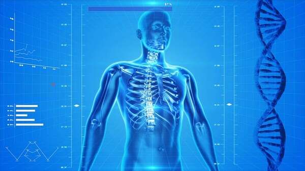
One of the primary areas where robots are already making significant strides is in diagnostics.
Imagine a robot capable of analyzing vast amounts of patient data, including medical history, genetic information, and real-time monitoring data. This robot can quickly identify potential health issues, predict disease risks, and recommend personalized treatment plans. With machine learning and artificial intelligence, these robots can continuously improve their diagnostic accuracy, ultimately saving lives by catching diseases at their earliest stages.
Let’s take a look at some companies that are currently involved in this market:
- Diagnostic Robotics: This company has developed an AI-powered platform that can be used to diagnose a wide range of diseases, including cancer, heart disease, and diabetes. The platform is currently being used by healthcare providers around the world.
- Paige AI: This company has developed AI-powered software that can be used to analyze pathology images and detect cancer cells. The software is currently being used by pathologists around the world to help them diagnose cancer more accurately and efficiently.
Robotic-assisted Surgery

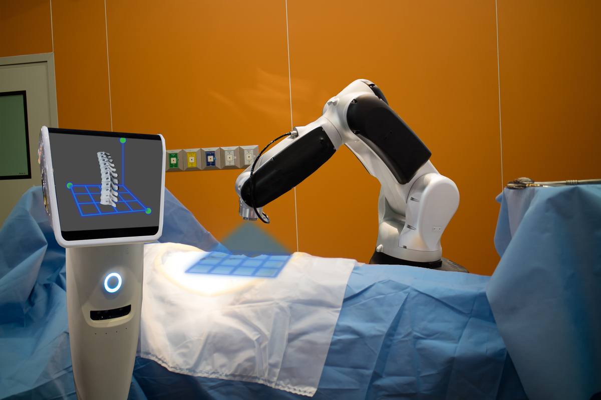
Robotic-assisted surgery is another promising frontier in healthcare. Robots equipped with advanced surgical instruments and guided by skilled surgeons can perform intricate procedures with unmatched precision and minimal invasiveness. These practices will reduce patient trauma, speed up recovery times, and lower the risk of complications.
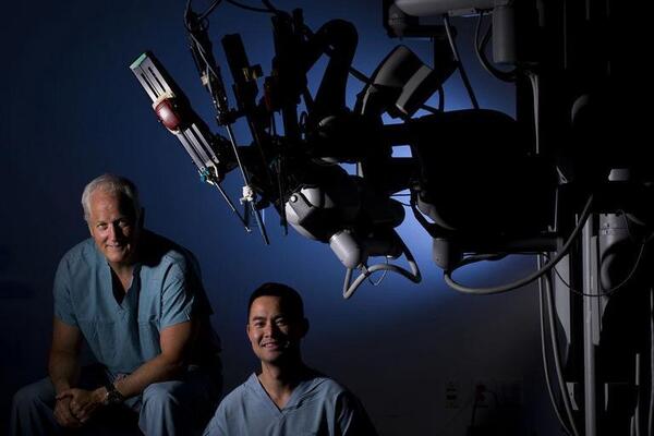
Also, robots can bridge geographical gaps by enabling remote surgery, allowing a surgeon in one location to operate on a patient in another, potentially saving lives in emergency situations and improving access to specialized care in remote areas.
Here are some of the leading companies involved in robotic-assisted surgery:
- Intuitive Surgical: Intuitive Surgical is the dominant player in the robotic-assisted surgery market, with its da Vinci surgical system being the most widely used robotic surgical system in the world.
- Medtronic: Medtronic recently entered the robotic-assisted surgery market with its Hugo robotic surgery system.
- Johnson & Johnson: Johnson & Johnson offers a variety of robotic surgery systems through its Johnson & Johnson Medical Devices division, including the Monarch platform for bronchoscopy, and the Velys platform for orthopedic surgery.
- Stryker: Stryker offers the Mako robotic-assisted surgery system for orthopedic surgery.
- Brainlab: Brainlab offers the Curve robotic-assisted surgery system for spinal and neurosurgery.
- CMR Surgical: CMR Surgical offers the Versius robotic-assisted surgery system for a variety of procedures, including general surgery, gynecologic surgery, and urologic surgery.
Enhanced Rehabilitation
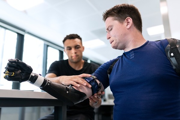
Rehabilitation is a cornerstone of healthcare, especially for patients recovering from injuries, surgeries, or chronic conditions. Robots are playing an increasingly important role in this area, providing consistent, personalized, and intensive therapy.
For example, robotic exoskeletons help patients regain mobility, while robotic arms assist those with limited dexterity. These devices not only enhance the quality of life for patients but also alleviate the strain on healthcare professionals by automating routine tasks, allowing them to focus on more complex aspects of care.
One of the first companies that comes to mind is ReWalk Robotics. ReWalk Robotics develops and manufactures robotic exoskeletons for people with spinal cord injuries.
ReWalk’s most well-known product is the ReWalk exoskeleton, which allows people with paraplegia to walk again. ReWalk Robotics also produces the ReStore exoskeleton, which is used to help people with lower limb disability regain their mobility.
Another company is Cyberdyne. Cyberdyne is a Japanese company that develops and manufactures robotic exoskeletons for medical and industrial use. Its most well-known product is the HAL (Hybrid Assistive Limb) exoskeleton, which is used to help people with disabilities walk, stand, and climb stairs. The HAL exoskeleton is also used in industrial settings to help workers lift heavy objects and perform other physically demanding tasks.
Robots in Patient Care
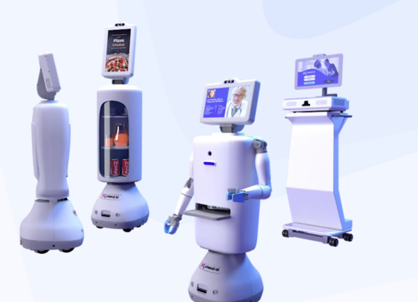
The future of healthcare also includes robots directly interacting with patients. Social robots equipped with natural language processing capabilities can provide companionship and emotional support to patients, particularly those in long-term care facilities or dealing with mental health issues. These robots can engage in conversations, give reminders when patients need to take medication, and monitor vital signs, ensuring patients receive the attention and care they need.
The company I work for, Xtend AI, is doing just that.
Pharmaceutical Advancements
In the pharmaceutical industry, robots are revolutionizing drug discovery and development. Robotic systems can automate high-throughput screening of compounds, drastically accelerating the process of identifying potential drug candidates.
Additionally, robots can handle complex chemical reactions with precision, leading to the creation of more effective and safe medications. This not only reduces the time and cost of drug development but also opens doors to personalized medicine, where treatments are tailored to individual patients based on their genetic makeup and health data.
One robot that already has a head start in this area is NiCoLA-B. This robot is used at the U.K. Center for Lead Discovery to test more than 300,000 compounds a day in search of promising drug candidates. It uses sound waves to move droplets of potential drugs into miniature wells on assay plates, where they are tested for activity.
Logistics and Supply Chain Management

Efficient logistics and supply chain management are critical in healthcare, ensuring that medications, medical equipment, and supplies are readily available when needed. Robots are already playing a pivotal role in this aspect by automating inventory management, drug dispensing, and even transportation within healthcare facilities. This not only reduces human errors but also optimizes resource allocation and minimizes wastage, ultimately leading to cost savings and improved patient care.
Challenges and Ethical Considerations
While the future of healthcare with robots is incredibly promising, it is not without its challenges and ethical considerations. Privacy concerns, data security, and the potential for bias in AI algorithms must be addressed. I predict there will always be a need for human oversight and expertise to ensure robots operate safely and effectively.
The Best is Yet to Come
The future impact of robots on healthcare is nothing short of transformative. From diagnostics and surgery to patient care and pharmaceutical advancements, robots are set to revolutionize every facet of the healthcare industry. As technology continues to advance, we can look forward to a healthcare system that is more efficient, accessible, and personalized, ultimately leading to better patient outcomes and an improved quality of life for all.
However, it is important we navigate this transformation with careful consideration of the ethical and privacy implications, ensuring that the benefits of healthcare robotics are realized while minimizing potential risks. The future of healthcare is indeed exciting, and robots will undoubtedly be at the forefront of this revolution.
Keep building!