Now that we’ve seen how to fill in Denavit-Hartenberg Tables, let’s see how we can use these tables and Python code to calculate homogeneous transformation matrices for robotic arms. Our goal is to then use these homogeneous transformation matrices to determine the position and orientation of the end effector of a robotic arm.

Example 1 – Cartesian Robot

Let’s start by calculating the homogeneous transformation matrix from frame 0 to frame 1.

Here was our derivation of the Denavit-Hartenberg table for the cartesian robot. Let’s enter that one in code. Here is the program in Python:

import numpy as np # Scientific computing library

# Project: Coding Denavit-Hartenberg Tables Using Python - Cartesian Robot
#          This only looks at frame 0 to frame 1.
# Author: Addison Sears-Collins
# Date created: August 21, 2020

# Link lengths in centimeters
a1 = 1 # Length of link 1
a2 = 1 # Length of link 2
a3 = 1 # Length of link 3

# Initialize values for the displacements
d1 = 1 # Displacement of link 1
d2 = 1 # Displacement of link 2
d3 = 1 # Displacement of link 3

# Declare the Denavit-Hartenberg table. 
# It will have four columns, to represent:
# theta, alpha, r, and d
# We have the convert angles to radians.
d_h_table = np.array([[np.deg2rad(90), np.deg2rad(90), 0, a1 + d1],
                      [np.deg2rad(90), np.deg2rad(-90), 0, a2 + d2],
                      [0, 0, 0, a3 + d3]]) 

# Create the homogeneous transformation matrix
homgen_0_1 = np.array([[np.cos(d_h_table[0,0]), -np.sin(d_h_table[0,0]) * np.cos(d_h_table[0,1]), np.sin(d_h_table[0,0]) * np.sin(d_h_table[0,1]), d_h_table[0,2] * np.cos(d_h_table[0,0])],
                      [np.sin(d_h_table[0,0]), np.cos(d_h_table[0,0]) * np.cos(d_h_table[0,1]), -np.cos(d_h_table[0,0]) * np.sin(d_h_table[0,1]), d_h_table[0,2] * np.sin(d_h_table[0,0])],
                      [0, np.sin(d_h_table[0,1]), np.cos(d_h_table[0,1]), d_h_table[0,3]],
                      [0, 0, 0, 1]])  

# Print the homogeneous transformation matrix from frame 1 to frame 0.
print(homgen_0_1)

Run the program.

Here is the output:

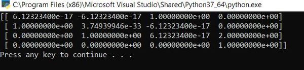
The output is saying that the rotation matrix from frame 0 to frame 1 is as follows:

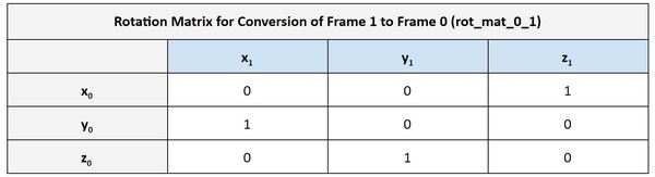
This is exactly what I got on an earlier post where I derived the rotation matrix from frame 0 to frame 1 for a cartesian robot.

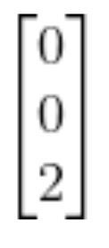
You can also see the displacement vector from frame 1 to frame 0, the 3×1 vector on the right side of the matrix. The vector makes sense because it is saying that the position of frame 1 relative to frame 0 in the z₀ direction is 2 units (because a₁ = 1 and d₁ = 1):

Now, let’s add the two other homogeneous transformation matrices: from frame 1 to 2 and from frame 2 to 3.

Here is the code:

import numpy as np # Scientific computing library

# Project: Coding Denavit-Hartenberg Tables Using Python - Cartesian Robot
# Author: Addison Sears-Collins
# Date created: August 21, 2020

# Link lengths in centimeters
a1 = 1 # Length of link 1
a2 = 1 # Length of link 2
a3 = 1 # Length of link 3

# Initialize values for the displacements
d1 = 1 # Displacement of link 1
d2 = 1 # Displacement of link 2
d3 = 1 # Displacement of link 3

# Declare the Denavit-Hartenberg table. 
# It will have four columns, to represent:
# theta, alpha, r, and d
# We have the convert angles to radians.
d_h_table = np.array([[np.deg2rad(90), np.deg2rad(90), 0, a1 + d1],
                      [np.deg2rad(90), np.deg2rad(-90), 0, a2 + d2],
                      [0, 0, 0, a3 + d3]]) 

# Homogeneous transformation matrix from frame 0 to frame 1
i = 0
homgen_0_1 = np.array([[np.cos(d_h_table[i,0]), -np.sin(d_h_table[i,0]) * np.cos(d_h_table[i,1]), np.sin(d_h_table[i,0]) * np.sin(d_h_table[i,1]), d_h_table[i,2] * np.cos(d_h_table[i,0])],
                      [np.sin(d_h_table[i,0]), np.cos(d_h_table[i,0]) * np.cos(d_h_table[i,1]), -np.cos(d_h_table[i,0]) * np.sin(d_h_table[i,1]), d_h_table[i,2] * np.sin(d_h_table[i,0])],
                      [0, np.sin(d_h_table[i,1]), np.cos(d_h_table[i,1]), d_h_table[i,3]],
                      [0, 0, 0, 1]])  

# Homogeneous transformation matrix from frame 1 to frame 2
i = 1
homgen_1_2 = np.array([[np.cos(d_h_table[i,0]), -np.sin(d_h_table[i,0]) * np.cos(d_h_table[i,1]), np.sin(d_h_table[i,0]) * np.sin(d_h_table[i,1]), d_h_table[i,2] * np.cos(d_h_table[i,0])],
                      [np.sin(d_h_table[i,0]), np.cos(d_h_table[i,0]) * np.cos(d_h_table[i,1]), -np.cos(d_h_table[i,0]) * np.sin(d_h_table[i,1]), d_h_table[i,2] * np.sin(d_h_table[i,0])],
                      [0, np.sin(d_h_table[i,1]), np.cos(d_h_table[i,1]), d_h_table[i,3]],
                      [0, 0, 0, 1]])  

# Homogeneous transformation matrix from frame 2 to frame 3
i = 2
homgen_2_3 = np.array([[np.cos(d_h_table[i,0]), -np.sin(d_h_table[i,0]) * np.cos(d_h_table[i,1]), np.sin(d_h_table[i,0]) * np.sin(d_h_table[i,1]), d_h_table[i,2] * np.cos(d_h_table[i,0])],
                      [np.sin(d_h_table[i,0]), np.cos(d_h_table[i,0]) * np.cos(d_h_table[i,1]), -np.cos(d_h_table[i,0]) * np.sin(d_h_table[i,1]), d_h_table[i,2] * np.sin(d_h_table[i,0])],
                      [0, np.sin(d_h_table[i,1]), np.cos(d_h_table[i,1]), d_h_table[i,3]],
                      [0, 0, 0, 1]])  

homgen_0_3 = homgen_0_1 @ homgen_1_2 @ homgen_2_3

# Print the homogeneous transformation matrices
print("Homogeneous Matrix Frame 0 to Frame 1:")
print(homgen_0_1)
print()
print("Homogeneous Matrix Frame 1 to Frame 2:")
print(homgen_1_2)
print()
print("Homogeneous Matrix Frame 2 to Frame 3:")
print(homgen_2_3)
print()
print("Homogeneous Matrix Frame 0 to Frame 3:")
print(homgen_0_3)
print()

Now, run the code.

Here is the output:

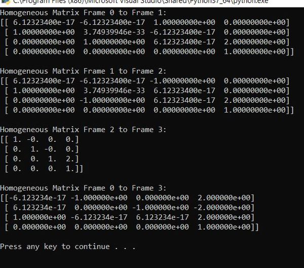
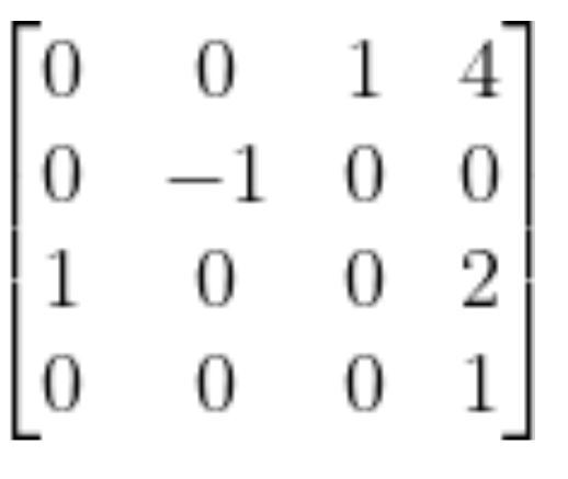
The homogeneous matrix from frame 0 to frame 3 is:

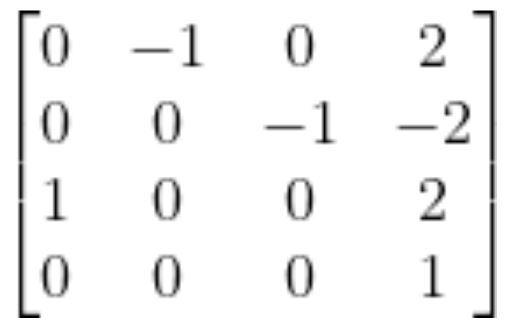
Let’s pull out the rotation matrix:

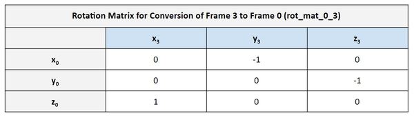
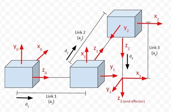
Let’s go through the matrix to see if it makes sense. Here is the diagram:

In the first column of the matrix, we see that the value on the third row is 1. It is saying that the x₃ vector is in the same direction as z₀. If we look at the diagram, we can see that this is in fact the case.

In the second column of the matrix, we see that the value on the first row is -1. It is saying that the y₃ vector is in the opposite direction as x₀. If we look at the diagram, we can see that this is in fact the case.

In the third column of the matrix, we see that the value on the second row is -1. It is saying that the z₃ vector is in the opposite direction as y₀. If we look at the diagram, we can see that this is in fact the case.

Finally, in the fourth column of the matrix, we have the displacement vector. Let’s pull that out.

6-displacement-vector-frame-3-to-frame-0JPG

The displacement vector portion of the matrix says that the position of the end effector of the robot is 2 units along x₀, -2 units along y₀, and 2 units along z₀. These results make sense given the link lengths and displacements were 1.

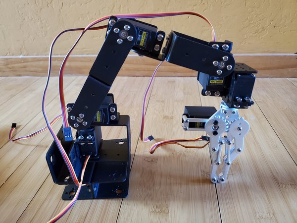
Example 2 – Six Degree of Freedom Robotic Arm

Let’s take a look at another example, a six degree of freedom robotic arm.

Here is the code:

import numpy as np # Scientific computing library

# Project: Coding Denavit-Hartenberg Tables Using Python - 6DOF Robotic Arm
#          This code excludes the servo motor that controls the gripper.
# Author: Addison Sears-Collins
# Date created: August 22, 2020

# Link lengths in centimeters
a1 = 1 # Length of link 1
a2 = 1 # Length of link 2
a3 = 1 # Length of link 3
a4 = 1 # Length of link 4
a5 = 1 # Length of link 5
a6 = 1 # Length of link 6

# Initialize values for the joint angles (degrees)
theta_1 = 0 # Joint 1
theta_2 = 0 # Joint 2
theta_3 = 0 # Joint 3
theta_4 = 0 # Joint 4
theta_5 = 0 # Joint 5

# Declare the Denavit-Hartenberg table. 
# It will have four columns, to represent:
# theta, alpha, r, and d
# We have the convert angles to radians.
d_h_table = np.array([[np.deg2rad(theta_1), np.deg2rad(90), 0, a1],
                      [np.deg2rad(theta_2), 0, a2, 0],
                      [np.deg2rad(theta_3), 0, a3, 0],
                      [np.deg2rad(theta_4 + 90), np.deg2rad(90), a5,0],
                      [np.deg2rad(theta_5), 0, 0, a4 + a6]]) 

# Homogeneous transformation matrix from frame 0 to frame 1
i = 0
homgen_0_1 = np.array([[np.cos(d_h_table[i,0]), -np.sin(d_h_table[i,0]) * np.cos(d_h_table[i,1]), np.sin(d_h_table[i,0]) * np.sin(d_h_table[i,1]), d_h_table[i,2] * np.cos(d_h_table[i,0])],
                      [np.sin(d_h_table[i,0]), np.cos(d_h_table[i,0]) * np.cos(d_h_table[i,1]), -np.cos(d_h_table[i,0]) * np.sin(d_h_table[i,1]), d_h_table[i,2] * np.sin(d_h_table[i,0])],
                      [0, np.sin(d_h_table[i,1]), np.cos(d_h_table[i,1]), d_h_table[i,3]],
                      [0, 0, 0, 1]])  

# Homogeneous transformation matrix from frame 1 to frame 2
i = 1
homgen_1_2 = np.array([[np.cos(d_h_table[i,0]), -np.sin(d_h_table[i,0]) * np.cos(d_h_table[i,1]), np.sin(d_h_table[i,0]) * np.sin(d_h_table[i,1]), d_h_table[i,2] * np.cos(d_h_table[i,0])],
                      [np.sin(d_h_table[i,0]), np.cos(d_h_table[i,0]) * np.cos(d_h_table[i,1]), -np.cos(d_h_table[i,0]) * np.sin(d_h_table[i,1]), d_h_table[i,2] * np.sin(d_h_table[i,0])],
                      [0, np.sin(d_h_table[i,1]), np.cos(d_h_table[i,1]), d_h_table[i,3]],
                      [0, 0, 0, 1]])  

# Homogeneous transformation matrix from frame 2 to frame 3
i = 2
homgen_2_3 = np.array([[np.cos(d_h_table[i,0]), -np.sin(d_h_table[i,0]) * np.cos(d_h_table[i,1]), np.sin(d_h_table[i,0]) * np.sin(d_h_table[i,1]), d_h_table[i,2] * np.cos(d_h_table[i,0])],
                      [np.sin(d_h_table[i,0]), np.cos(d_h_table[i,0]) * np.cos(d_h_table[i,1]), -np.cos(d_h_table[i,0]) * np.sin(d_h_table[i,1]), d_h_table[i,2] * np.sin(d_h_table[i,0])],
                      [0, np.sin(d_h_table[i,1]), np.cos(d_h_table[i,1]), d_h_table[i,3]],
                      [0, 0, 0, 1]])  

# Homogeneous transformation matrix from frame 3 to frame 4
i = 3
homgen_3_4 = np.array([[np.cos(d_h_table[i,0]), -np.sin(d_h_table[i,0]) * np.cos(d_h_table[i,1]), np.sin(d_h_table[i,0]) * np.sin(d_h_table[i,1]), d_h_table[i,2] * np.cos(d_h_table[i,0])],
                      [np.sin(d_h_table[i,0]), np.cos(d_h_table[i,0]) * np.cos(d_h_table[i,1]), -np.cos(d_h_table[i,0]) * np.sin(d_h_table[i,1]), d_h_table[i,2] * np.sin(d_h_table[i,0])],
                      [0, np.sin(d_h_table[i,1]), np.cos(d_h_table[i,1]), d_h_table[i,3]],
                      [0, 0, 0, 1]])  

# Homogeneous transformation matrix from frame 4 to frame 5
i = 4
homgen_4_5 = np.array([[np.cos(d_h_table[i,0]), -np.sin(d_h_table[i,0]) * np.cos(d_h_table[i,1]), np.sin(d_h_table[i,0]) * np.sin(d_h_table[i,1]), d_h_table[i,2] * np.cos(d_h_table[i,0])],
                      [np.sin(d_h_table[i,0]), np.cos(d_h_table[i,0]) * np.cos(d_h_table[i,1]), -np.cos(d_h_table[i,0]) * np.sin(d_h_table[i,1]), d_h_table[i,2] * np.sin(d_h_table[i,0])],
                      [0, np.sin(d_h_table[i,1]), np.cos(d_h_table[i,1]), d_h_table[i,3]],
                      [0, 0, 0, 1]])  

homgen_0_5 = homgen_0_1 @ homgen_1_2 @ homgen_2_3 @ homgen_3_4 @ homgen_4_5 

# Print the homogeneous transformation matrices
print("Homogeneous Matrix Frame 0 to Frame 5:")
print(homgen_0_5)

Now, run the code:

Here is the output:

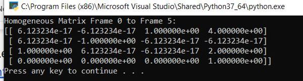
In matrix form, this is:

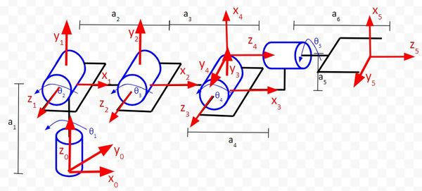
Does this make sense? Here is the diagram:

In the first column of the matrix, we see that the value on the third row is 1. It is saying that the x₅ vector is in the same direction as z₀. If we look at the diagram, we can see that this is in fact the case.

In the second column of the matrix, we see that the value on the second row is -1. It is saying that the y₅ vector is in the opposite direction as y₀. If we look at the diagram, we can see that this is in fact the case.

In the third column of the matrix, we see that the value on the first row is 1. It is saying that the z₅ vector is in the same direction as x₀. If we look at the diagram, we can see that this is in fact the case.

Finally, in the fourth column of the matrix, we have the displacement vector. This portion of the matrix says that the position of the end effector of the robot is 4 units along x₀, 0 units along y₀, and 2 units along z₀. These results make sense given that we set all the link lengths to 1.

References

Credit to Professor Angela Sodemann from whom I learned these important robotics fundamentals. Dr. Sodemann teaches robotics over at her website, RoboGrok.com. While she uses the PSoC in her work, I use Arduino and Raspberry Pi since I’m more comfortable with these computing platforms. Angela is an excellent teacher and does a fantastic job explaining various robotics topics over on her YouTube channel.