In this post, I will show you some useful world files that you can use in your ROS 2/Gazebo robotics development work. 

All of these world files have been tested on my machine.

A lot of these world files were originally missing key models and other mesh files when I downloaded them from GitHub and loaded them on my machine…so I spent several (at times, frustrating) days fixing those issues to save you a lot of headache.

Prerequisites

• ROS 2 Foxy Fitzroy installed on Ubuntu Linux 20.04 or newer. I am using ROS 2 Galactic, which is the latest version of ROS 2 as of the date of this post.
• You have already created a ROS 2 workspace. The name of our workspace is “dev_ws”, which stands for “development workspace.” 
• (Optional) You have a package named two_wheeled_robot inside your ~/dev_ws/src folder, which I set up in this post. If you have another package, that is fine.
• You know how to load a world file into Gazebo using ROS 2.

Link to the World and Models Files

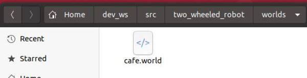
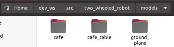
You can find the files for all worlds and models (which are the objects inside those worlds) here on my Google Drive. Check the ‘worlds’ and ‘models’ folder of my two_wheeled_robot package.

Useful Command

To switch between world files when you are loading a world into Gazebo using a ROS 2 launch file, you can use the following command (all this command goes on one line):

ros2 launch <package_name> <launch_file_name.py> world:=<path_to_world_file>

For example:

ros2 launch two_wheeled_robot load_world_into_gazebo.launch.py world:=~/dev_ws/src/two_wheeled_robot_worlds/cafe.world

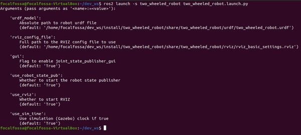
ROS 2 Launch File

Here is what my launch file looks like:

# Author: Addison Sears-Collins
# Date: September 23, 2021
# Description: Load a world file into Gazebo.
# https://automaticaddison.com

import os
from launch import LaunchDescription
from launch.actions import DeclareLaunchArgument, IncludeLaunchDescription
from launch.conditions import IfCondition, UnlessCondition
from launch.launch_description_sources import PythonLaunchDescriptionSource
from launch.substitutions import Command, LaunchConfiguration, PythonExpression
from launch_ros.actions import Node
from launch_ros.substitutions import FindPackageShare

def generate_launch_description():

  # Set the path to the Gazebo ROS package
  pkg_gazebo_ros = FindPackageShare(package='gazebo_ros').find('gazebo_ros')   
  
  # Set the path to this package.
  pkg_share = FindPackageShare(package='two_wheeled_robot').find('two_wheeled_robot')

  # Set the path to the world file
  world_file_name = 'warehouse.world'
  world_path = os.path.join(pkg_share, 'worlds', world_file_name)
  
  # Set the path to the SDF model files.
  gazebo_models_path = os.path.join(pkg_share, 'models')
  os.environ["GAZEBO_MODEL_PATH"] = gazebo_models_path

  ########### YOU DO NOT NEED TO CHANGE ANYTHING BELOW THIS LINE ##############  
  # Launch configuration variables specific to simulation
  headless = LaunchConfiguration('headless')
  use_sim_time = LaunchConfiguration('use_sim_time')
  use_simulator = LaunchConfiguration('use_simulator')
  world = LaunchConfiguration('world')

  declare_simulator_cmd = DeclareLaunchArgument(
    name='headless',
    default_value='False',
    description='Whether to execute gzclient')
    
  declare_use_sim_time_cmd = DeclareLaunchArgument(
    name='use_sim_time',
    default_value='true',
    description='Use simulation (Gazebo) clock if true')

  declare_use_simulator_cmd = DeclareLaunchArgument(
    name='use_simulator',
    default_value='True',
    description='Whether to start the simulator')

  declare_world_cmd = DeclareLaunchArgument(
    name='world',
    default_value=world_path,
    description='Full path to the world model file to load')
   
  # Specify the actions
  
  # Start Gazebo server
  start_gazebo_server_cmd = IncludeLaunchDescription(
    PythonLaunchDescriptionSource(os.path.join(pkg_gazebo_ros, 'launch', 'gzserver.launch.py')),
    condition=IfCondition(use_simulator),
    launch_arguments={'world': world}.items())

  # Start Gazebo client    
  start_gazebo_client_cmd = IncludeLaunchDescription(
    PythonLaunchDescriptionSource(os.path.join(pkg_gazebo_ros, 'launch', 'gzclient.launch.py')),
    condition=IfCondition(PythonExpression([use_simulator, ' and not ', headless])))

  # Create the launch description and populate
  ld = LaunchDescription()

  # Declare the launch options
  ld.add_action(declare_simulator_cmd)
  ld.add_action(declare_use_sim_time_cmd)
  ld.add_action(declare_use_simulator_cmd)
  ld.add_action(declare_world_cmd)

  # Add any actions
  ld.add_action(start_gazebo_server_cmd)
  ld.add_action(start_gazebo_client_cmd)

  return ld

Worlds

Cafe World

I showed you how to load the cafe.world file in this post. Here are the files for that. You can use this world to test an indoor delivery robot that can deliver food and drinks to a table.

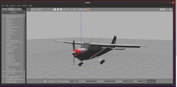
Car World

Let’s build a world for a car to move around in. Credit to this GitHub repository for the model and world files. You can use this world to test autonomous vehicle algorithms.

Here is how it looks:

Distribution Center World

Let’s create a distribution center world. Credit to this GitHub repository for the model and world files. You can use this world to test autonomous mobile robots.

Here is how it looks:

Factory World

Let’s create a factory world. Credit to this GitHub repository for the model and world files. You can use this world to test autonomous mobile robots.

Here is how it looks:

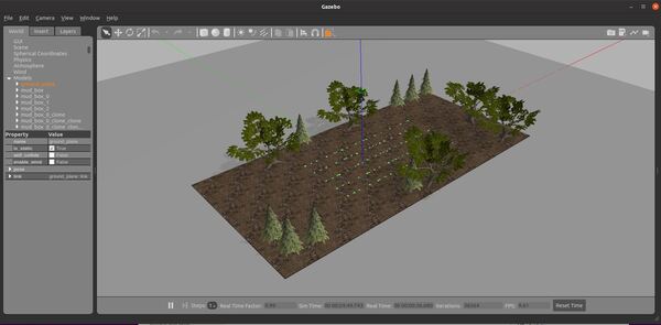
Farm World

Let’s create a farm world. Credit to this GitHub repository for the model files. You can use this world to test autonomous weeding machines or tractors for agricultural robotics work.

Here is how it looks:

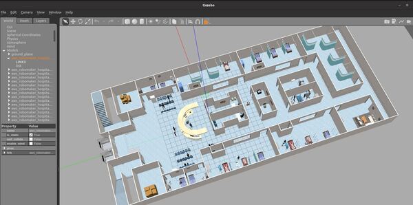
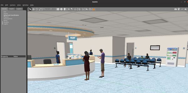
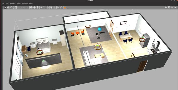
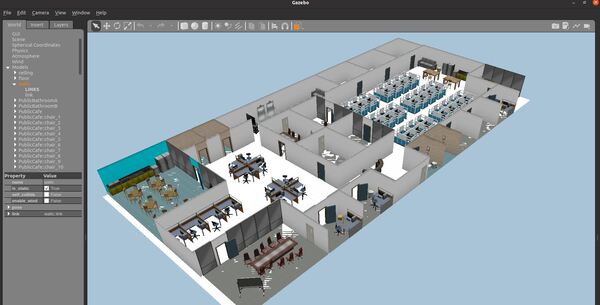
Hospital World

Let’s create a hospital world. Credit to this GitHub repository for the model and world files. You can use these worlds to test indoor delivery robots or mobile disinfection robots.

Here is how it looks:

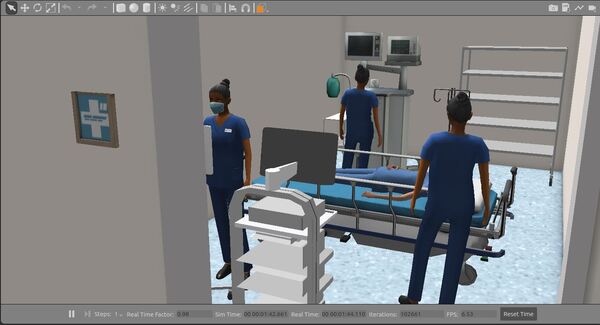
Here is how it looks with two floors:

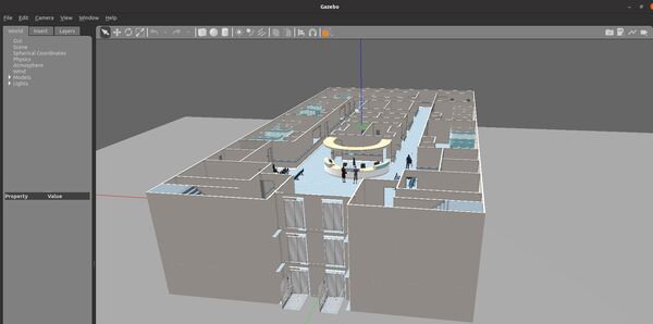
Here is how it looks with three floors:

House World

Let’s create a hospital world. Credit to this GitHub repository for the model and world files. You can use this world to test autonomous vacuum cleaners or other household robots.

Here is how it looks:

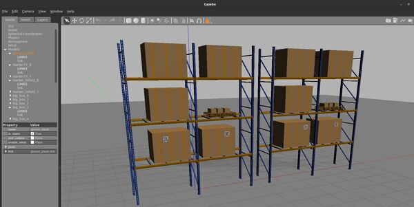
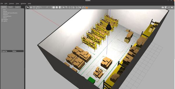
Inventory World

Let’s create an inventory world. You can use this world to create QR scanning drones that can perform inventory management in a warehouse. Credit to this GitHub repository for the model and world files.

Here is how it looks:

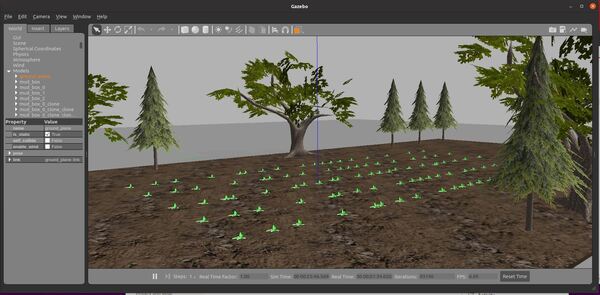
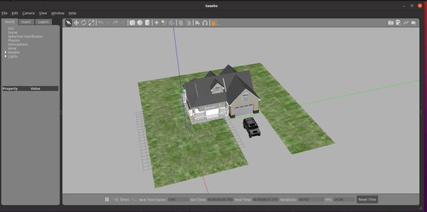
Lawn World

Here is what my lawn world looks like. You could use this simulated world to test autonomous lawnmower algorithms.

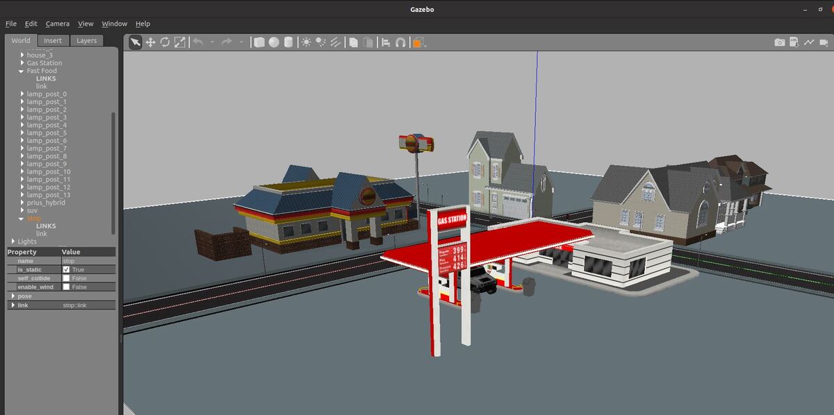
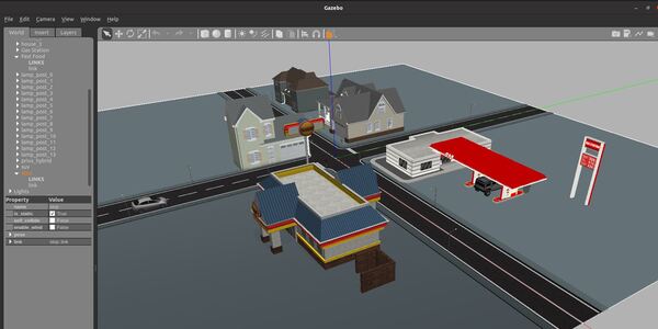
Neighborhood World

Let’s create a neighborhood world. Credit to this GitHub repository for the world file. You can use this world to test outdoor delivery robots.

Here is how it looks:

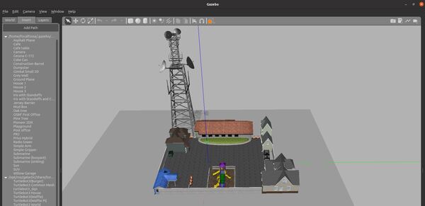
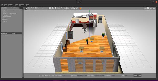
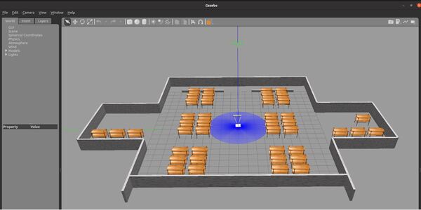
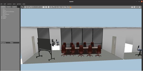
Office World

Let’s create an office world. Credit to this GitHub repository for the world file. You can use this world to test indoor delivery robots.

Go to your media folder of Gazebo.

cd /usr/share/gazebo-11/media

Make a meshes folder.

sudo mkdir meshes

Add these meshes to the folder. The command below goes all on one line inside the Linux terminal.

sudo cp ~/dev_ws/src/two_wheeled_robot/meshes/office/* /usr/share/gazebo-11/media/meshes

Now copy the media files (both the scripts and textures).

sudo cp ~/dev_ws/src/two_wheeled_robot/media/materials/scripts/* /usr/share/gazebo-11/media/materials/scripts

sudo cp ~/dev_ws/src/two_wheeled_robot/media/materials/textures/* /usr/share/gazebo-11/media/materials/textures

Make sure your models folder has all these models.

Add the office.world file to your worlds folder.

Modify the launch file and launch the world.

Here is how the world looks:

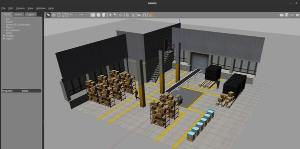
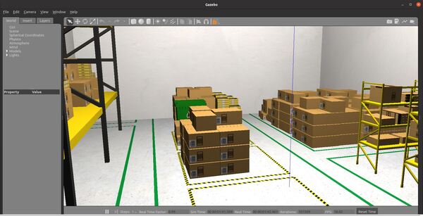
Warehouse World

Let’s create a warehouse world. Credit to this GitHub repository for the model and world files. You can use this world to test autonomous mobile robots that move pallets and shelves around the warehouse floor.

Here is how it looks:

That’s it. Keep building!

In this tutorial, I will show you how to load a .world file into Gazebo. 

You can learn all about world files at this link.

Real-World Applications

Simulating a world has a number of real-world robotic applications: 

• Ground Delivery
• Hospitals and Medical Centers
• Hotels (Room Service)
• Offices
• Restaurants
• Warehouses
• And more…

Roboticists like to simulate robots in simulated worlds in order to test out different algorithms. You can imagine the cost of making mistakes with a physical robot can be high (e.g. crashing a mobile robot into a wall at high speed means lost money).

You can get all the code for this tutorial here.

Let’s get started!

Prerequisites

• ROS 2 Foxy Fitzroy installed on Ubuntu Linux 20.04 or newer. I am using ROS 2 Galactic, which is the latest version of ROS 2 as of the date of this post.
  • If you are using another ROS 2 distribution, you will need to replace ‘galactic’ with the name of your distribution everywhere I mention ‘galactic’ in this tutorial. 
  • I highly recommend you get the newest version of ROS 2. If you are using a newer version of ROS 2, you can still follow all the steps in this tutorial. Everything will work just fine.
• You have already created a ROS 2 workspace. The name of our workspace is “dev_ws”, which stands for “development workspace.” 
• (Optional) You have a package named two_wheeled_robot inside your ~/dev_ws/src folder, which I set up in this post. If you have another package, that is fine.

Manually 

Quick Start

The easiest way to load a world is via the command line. 

Open a new terminal window.

Type the following command to open up a world named cafe.world. This file is one of the built-in worlds that comes with the Gazebo installation (I am using Gazebo 11).

gazebo worlds/cafe.world

You can see a list of all the built-in worlds in this GitHub repository.

The world files are located in your /usr/share/gazebo-11/worlds directory.

The models (i.e. models for the objects that are inside your world) are located inside this directory:

~/.gazebo/models

Where focalfossa is the name of your Linux environment.

When you want to close the world, go back to the terminal, and type:

CTRL + C

Your Own World

If you have your own world, you can follow the instructions on this post to test it in Gazebo.

Alternatively, you can launch Gazebo using the following command.

gazebo

Then go to the Insert tab, and start inserting items inside the empty world. 

Once you’re done, you can save the world file by going to File ->Save World As.

Using a Launch File

Example – Cafe World

Let’s launch the cafe world we saw earlier using a ROS 2 launch file.

I want to copy the cafe.world file to the worlds folder of my ROS 2 package.

cd /usr/share/gazebo-11/worlds

cp cafe.world ~/dev_ws/src/two_wheeled_robot/worlds

The syntax is:

cp <world file> <path to the worlds folder inside your ROS 2 package>

cd ~/dev_ws/src/two_wheeled_robot/worlds

gedit cafe.world

You will see the cafe.world file has various links to other models and mesh files in it. Let’s move those files over to our package so that everything is all inside our two_wheeled_robot package (or whatever ROS 2 package you’re using).

Start from the top of the cafe.world file.

The first model we need to move over is the ground_plane model.

cd ~/.gazebo/models

cp -r ground_plane ~/dev_ws/src/two_wheeled_robot/models

Now let’s copy over the other models.

cp -r cafe ~/dev_ws/src/two_wheeled_robot/models

cp -r cafe_table ~/dev_ws/src/two_wheeled_robot/models

Now let’s create a launch file.

colcon_cd two_wheeled_robot

cd launch

gedit load_world_into_gazebo.launch.py

Write this code inside the file.

# Author: Addison Sears-Collins
# Date: September 19, 2021
# Description: Load a world file into Gazebo.
# https://automaticaddison.com

import os
from launch import LaunchDescription
from launch.actions import DeclareLaunchArgument, IncludeLaunchDescription
from launch.conditions import IfCondition, UnlessCondition
from launch.launch_description_sources import PythonLaunchDescriptionSource
from launch.substitutions import Command, LaunchConfiguration, PythonExpression
from launch_ros.actions import Node
from launch_ros.substitutions import FindPackageShare

def generate_launch_description():

  # Set the path to the Gazebo ROS package
  pkg_gazebo_ros = FindPackageShare(package='gazebo_ros').find('gazebo_ros')   
  
  # Set the path to this package.
  pkg_share = FindPackageShare(package='two_wheeled_robot').find('two_wheeled_robot')

  # Set the path to the world file
  world_file_name = 'cafe.world'
  world_path = os.path.join(pkg_share, 'worlds', world_file_name)
  
  # Set the path to the SDF model files.
  gazebo_models_path = os.path.join(pkg_share, 'models')
  os.environ["GAZEBO_MODEL_PATH"] = gazebo_models_path

  ########### YOU DO NOT NEED TO CHANGE ANYTHING BELOW THIS LINE ##############  
  # Launch configuration variables specific to simulation
  headless = LaunchConfiguration('headless')
  use_sim_time = LaunchConfiguration('use_sim_time')
  use_simulator = LaunchConfiguration('use_simulator')
  world = LaunchConfiguration('world')

  declare_simulator_cmd = DeclareLaunchArgument(
    name='headless',
    default_value='False',
    description='Whether to execute gzclient')
    
  declare_use_sim_time_cmd = DeclareLaunchArgument(
    name='use_sim_time',
    default_value='true',
    description='Use simulation (Gazebo) clock if true')

  declare_use_simulator_cmd = DeclareLaunchArgument(
    name='use_simulator',
    default_value='True',
    description='Whether to start the simulator')

  declare_world_cmd = DeclareLaunchArgument(
    name='world',
    default_value=world_path,
    description='Full path to the world model file to load')
   
  # Specify the actions
  
  # Start Gazebo server
  start_gazebo_server_cmd = IncludeLaunchDescription(
    PythonLaunchDescriptionSource(os.path.join(pkg_gazebo_ros, 'launch', 'gzserver.launch.py')),
    condition=IfCondition(use_simulator),
    launch_arguments={'world': world}.items())

  # Start Gazebo client    
  start_gazebo_client_cmd = IncludeLaunchDescription(
    PythonLaunchDescriptionSource(os.path.join(pkg_gazebo_ros, 'launch', 'gzclient.launch.py')),
    condition=IfCondition(PythonExpression([use_simulator, ' and not ', headless])))

  # Create the launch description and populate
  ld = LaunchDescription()

  # Declare the launch options
  ld.add_action(declare_simulator_cmd)
  ld.add_action(declare_use_sim_time_cmd)
  ld.add_action(declare_use_simulator_cmd)
  ld.add_action(declare_world_cmd)

  # Add any actions
  ld.add_action(start_gazebo_server_cmd)
  ld.add_action(start_gazebo_client_cmd)

  return ld

Save the file, and close it.

Go to your root directory.

cd ~/dev_ws

Build the package.

colcon build

Open a new terminal window.

Run the launch file using the following command:

ros2 launch two_wheeled_robot load_world_into_gazebo.launch.py

Here is the output. You should see the actors walking around the cafe.

Summary

In summary, the procedure for creating a world entails the following steps:

1. Create the .world file inside the worlds folder of your package.
2. Add the SDF models to the models folder of your package.
3. Edit the launch file.
4. Build the package.
5. Launch the world.

In this tutorial, I will show you how to load a URDF File into RViz. Universal Robot Description Format (URDF) is the standard ROS format for robot modeling.

Prerequisites

• ROS 2 Foxy Fitzroy installed on Ubuntu Linux 20.04 
  • If you are using another ROS 2 distribution, you will need to replace ‘foxy’ with the name of your distribution everywhere I mention ‘foxy’ in this tutorial. 
  • I highly recommend you get the newest version of ROS 2. If you are using a newer version of ROS 2, you can still follow all the steps in this tutorial.
• You have already created a ROS 2 workspace. The name of our workspace is “dev_ws”, which stands for “development workspace.”

You can find the entire code for this project here on my Google Drive.

What is URDF?

A URDF (Universal Robot Description Format) file is an XML file that describes what a robot should look like in real life. It contains the complete physical description of the robot.

You can learn more about URDF files here.

Install Important ROS 2 Packages

First, we need to install some important ROS 2 packages that we will use in this tutorial. Open a new terminal window, and type the following commands, one right after the other.

sudo apt install ros-foxy-joint-state-publisher-gui

sudo apt install ros-foxy-xacro

The format of the commands above is:

sudo apt install ros-<ros2-distro>-joint-state-publisher-gui

sudo apt install ros-<ros2-distro>-xacro

You will need to replace <ros2-distro> with the ROS 2 distribution you are using. In this case, I am using ROS 2 Foxy Fitzroy, which is ‘foxy’ for short.

Create a ROS 2 Package

Let’s create a ROS 2 package inside our workspace. My workspace is named dev_ws.

In a new terminal window, move to the src (source) folder of your workspace.

cd ~/dev_ws/src

Now create the package using the following command.

ros2 pkg create --build-type ament_cmake two_wheeled_robot

Create Extra Folders

Move inside the package.

cd ~/dev_ws/src/two_wheeled_robot/

Create some extra folders with the following names. We will not use all of these folders. I just like to have these folders in every package I create in case I need to use them.

mkdir config launch maps meshes models params rviz urdf worlds

Type the following command to verify the folders were created.

dir

Now build the package by typing the following command:

cd ~/dev_ws

colcon build

Let’s add a script to our bashrc file which enables us to use the following command to move to the package from any directory inside our terminal window.

colcon_cd two_wheeled_robot

Where ‘cd’ means “change directory”.

Note that in ROS 1, we typed roscd to change directories. In ROS 2, we use the colcon_cd command instead of roscd.

Open a terminal window, and type the following commands, one right after the other:

echo "source /usr/share/colcon_cd/function/colcon_cd.sh" >> ~/.bashrc

echo "export _colcon_cd_root=~/dev_ws" >> ~/.bashrc

Now open a new terminal window.

To go directly to the basic_mobile_robot ROS 2 package, type:

colcon_cd two_wheeled_robot

This command above will get you straight to the two_wheeled_robot package from within any directory in your Linux system. The format is:

colcon_cd [ROS 2 package name]

Create the URDF File

In this section, we will build our mobile robot step-by-step. Our robot will be defined in a Universal Robot Descriptor File (URDF), the XML file that represents a robot model.

Open a new terminal window, and type:

colcon_cd two_wheeled_robot

cd urdf

Make sure you have the Gedit text editor installed.

sudo apt-get install gedit

Create a new file named two_wheeled_robot.urdf.

gedit two_wheeled_robot.urdf

Inside this file, we define what our robot will look like (i.e. visual properties), how the robot will behave when it bumps into stuff (i.e. collision properties), and its mass (i.e. inertial properties). 

Type this code inside the URDF file.

Save and close the file.

Now go to the meshes folder.

cd ~/dev_ws/src/two_wheeled_robot/meshes

Add this STL file to your meshes folder. A mesh is a file that allows your robot to look more realistic (rather than just using basic shapes like boxes and spheres).

Rather than use the STL files I provided, you can use a program like SolidWorks to generate your own STL files. You can also use a program called Blender to create DAE files. URDF files support meshes in either STL or DAE format.

Add Dependencies

Let’s add some packages that our project will depend on. Go to the package.xml file.

cd ~/dev_ws/src/two_wheeled_robot/

OR

colcon_cd two_wheeled_robot 

gedit package.xml

After the <buildtool_depend> tag, add the following lines:

<exec_depend>joint_state_publisher</exec_depend>
<exec_depend>robot_state_publisher</exec_depend>
<exec_depend>rviz</exec_depend>
<exec_depend>xacro</exec_depend>

Save the file, and close it.

We will be using the Joint State Publisher and the Robot State Publisher. We will also be using RViz to visualize our robot model.

Create the Launch File

Let’s create a launch file. Open a new terminal window, and type:

colcon_cd two_wheeled_robot

cd launch

gedit two_wheeled_robot.launch.py

Copy and paste this code into the file.

# Author: Addison Sears-Collins
# Date: September 14, 2021
# Description: Launch a two-wheeled robot URDF file using Rviz.
# https://automaticaddison.com

import os
from launch import LaunchDescription
from launch.actions import DeclareLaunchArgument
from launch.conditions import IfCondition, UnlessCondition
from launch.substitutions import Command, LaunchConfiguration
from launch_ros.actions import Node
from launch_ros.substitutions import FindPackageShare

def generate_launch_description():

  # Set the path to this package.
  pkg_share = FindPackageShare(package='two_wheeled_robot').find('two_wheeled_robot')

  # Set the path to the RViz configuration settings
  default_rviz_config_path = os.path.join(pkg_share, 'rviz/rviz_basic_settings.rviz')

  # Set the path to the URDF file
  default_urdf_model_path = os.path.join(pkg_share, 'urdf/two_wheeled_robot.urdf')

  ########### YOU DO NOT NEED TO CHANGE ANYTHING BELOW THIS LINE ##############  
  # Launch configuration variables specific to simulation
  gui = LaunchConfiguration('gui')
  urdf_model = LaunchConfiguration('urdf_model')
  rviz_config_file = LaunchConfiguration('rviz_config_file')
  use_robot_state_pub = LaunchConfiguration('use_robot_state_pub')
  use_rviz = LaunchConfiguration('use_rviz')
  use_sim_time = LaunchConfiguration('use_sim_time')

  # Declare the launch arguments  
  declare_urdf_model_path_cmd = DeclareLaunchArgument(
    name='urdf_model', 
    default_value=default_urdf_model_path, 
    description='Absolute path to robot urdf file')
    
  declare_rviz_config_file_cmd = DeclareLaunchArgument(
    name='rviz_config_file',
    default_value=default_rviz_config_path,
    description='Full path to the RVIZ config file to use')
    
  declare_use_joint_state_publisher_cmd = DeclareLaunchArgument(
    name='gui',
    default_value='True',
    description='Flag to enable joint_state_publisher_gui')
  
  declare_use_robot_state_pub_cmd = DeclareLaunchArgument(
    name='use_robot_state_pub',
    default_value='True',
    description='Whether to start the robot state publisher')

  declare_use_rviz_cmd = DeclareLaunchArgument(
    name='use_rviz',
    default_value='True',
    description='Whether to start RVIZ')
    
  declare_use_sim_time_cmd = DeclareLaunchArgument(
    name='use_sim_time',
    default_value='True',
    description='Use simulation (Gazebo) clock if true')
   
  # Specify the actions

  # Publish the joint state values for the non-fixed joints in the URDF file.
  start_joint_state_publisher_cmd = Node(
    condition=UnlessCondition(gui),
    package='joint_state_publisher',
    executable='joint_state_publisher',
    name='joint_state_publisher')

  # A GUI to manipulate the joint state values
  start_joint_state_publisher_gui_node = Node(
    condition=IfCondition(gui),
    package='joint_state_publisher_gui',
    executable='joint_state_publisher_gui',
    name='joint_state_publisher_gui')

  # Subscribe to the joint states of the robot, and publish the 3D pose of each link.
  start_robot_state_publisher_cmd = Node(
    condition=IfCondition(use_robot_state_pub),
    package='robot_state_publisher',
    executable='robot_state_publisher',
    parameters=[{'use_sim_time': use_sim_time, 
    'robot_description': Command(['xacro ', urdf_model])}],
    arguments=[default_urdf_model_path])

  # Launch RViz
  start_rviz_cmd = Node(
    condition=IfCondition(use_rviz),
    package='rviz2',
    executable='rviz2',
    name='rviz2',
    output='screen',
    arguments=['-d', rviz_config_file])
  
  # Create the launch description and populate
  ld = LaunchDescription()

  # Declare the launch options
  ld.add_action(declare_urdf_model_path_cmd)
  ld.add_action(declare_rviz_config_file_cmd)
  ld.add_action(declare_use_joint_state_publisher_cmd)
  ld.add_action(declare_use_robot_state_pub_cmd)  
  ld.add_action(declare_use_rviz_cmd) 
  ld.add_action(declare_use_sim_time_cmd)

  # Add any actions
  ld.add_action(start_joint_state_publisher_cmd)
  ld.add_action(start_joint_state_publisher_gui_node)
  ld.add_action(start_robot_state_publisher_cmd)
  ld.add_action(start_rviz_cmd)

  return ld

Save the file, and close it.

You can read more about Launch files here.

Add the RViz Configuration File

Let’s add a configuration file that will initialize RViz with the proper settings so we can view the robot as soon as RViz launches.

Open a new terminal window. Type:

colcon_cd two_wheeled_robot

cd rviz

gedit rviz_basic_settings.rviz

Add this code.

Save the file, and close it.

Build the Package

Now we need to build the package. Open a new terminal window, and type:

colcon_cd two_wheeled_robot

gedit CMakeLists.txt

Add the following snippet to CMakeLists.txt file above the if(BUILD_TESTING) line.

install(
  DIRECTORY config launch maps meshes models params rviz src urdf worlds
  DESTINATION share/${PROJECT_NAME}
)

Save the file and close it.

Build the project.

cd ~/dev_ws/

colcon build

In the future, if you would like to build the two_wheeled_robot package only, you can type:

colcon build --packages-select two_wheeled_robot

Launch the Robot in RViz

Open a new terminal, and launch the robot.

cd ~/dev_ws/

ros2 launch two_wheeled_robot two_wheeled_robot.launch.py

——

By the way, if you want to see the available arguments you can pass to the launch file from the terminal window, type:

ros2 launch -s two_wheeled_robot two_wheeled_robot.launch.py

And if you want to set the value of an argument (e.g. launch the robot without RViz), you can do something like this:

ros2 launch two_wheeled_robot two_wheeled_robot.launch.py use_rviz:='False'

——

Here is the output after we launch the robot in RViz:

The joint state publisher GUI has sliders that enable you to move the wheels.

If something goes wrong with the launch, close everything down, restart Linux, and launch again.

Check whether you have properly set up the collision properties by enabling Collision Enabled under RobotModel on the left pane.

You can see in the image that I have modeled the base_link as a box for collisions. I could have just as easily used the STL model itself (which was used for visualization) as the collision geometry, but I decided to go with the simpler box representation to give me more flexibility to alter the collision areas if necessary. Also, Gazebo (a popular robotics simulator) recommends using simpler collision geometry to increase performance.

View the Coordinate Frames

Let’s see the coordinate frames. We first need to install the necessary software.

sudo apt install ros-foxy-tf2-tools

Check out the coordinate frames.

colcon_cd two_wheeled_robot

ros2 run tf2_tools view_frames.py

As of ROS Galactic, this command is:

ros2 run tf2_tools view_frames

In the current working directory, you will have a file called frames.pdf. Open that file.

evince frames.pdf

Here is what my coordinate transform (i.e. tf) tree looks like:

If we want to see the coordinate transformation from one link to another, we can type the following command. For example, what is the position and orientation of the front caster wheel relative to the base_link of the robot?

The syntax is:

ros2 run tf2_ros tf2_echo <parent frame> <child frame>

We open a terminal window, and type:

ros2 run tf2_ros tf2_echo base_link front_caster

Here is the output. With respect to the base_link reference frame, the front caster wheel is located at (x=0.217 meters, y=0 meters, and z=-0.1 meters). 

The rotation value is in quaternion format. You can see that the rotation values are all 0s, indicating that the orientation of both coordinate frames is equivalent (i.e. the x, y, and z axes of both coordinate frames point in the same direction).

Remember that, by convention:

• x-axis is red
• y-axis is green
• z-axis is blue 

To see an image of the architecture of our ROS system, open a new terminal window, and type the following command:

rqt_graph

Select the “Nodes/Topics (all) option in the upper-left part of the screen, and then click the refresh arrow right next to it.

You can see how the joint state publisher GUI manipulates the joint states (i.e. the angle of each wheel joint). This data feeds into the robot state publisher. The robot state publisher publishes the coordinate frame relationships to tf, and the updated robot model feeds into RViz, the robot model visualization program.

That’s it! 

When you’re done, press CTRL+C in all terminal windows to shut everything down.