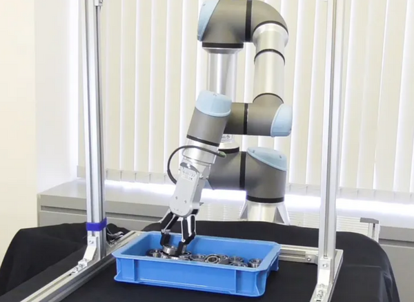
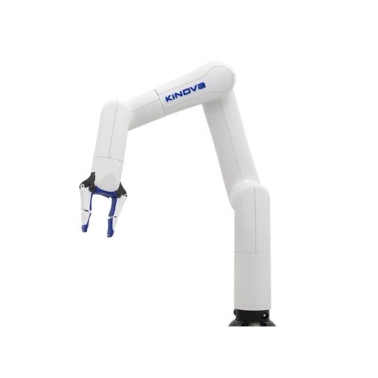
In this tutorial, I’ll show you how to use ROS 2 and RViz to visualize the Gen3 Lite Robot by Kinova Robotics.
Prerequisites
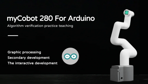
- (Optional) You have completed this tutorial in which I build a URDF file from scratch for the myCobot 280 by Elephant Robotics.
Useful Links
Here is my GitHub repository for this robotic arm. All the files we will create in this tutorial are also stored there.
Below are some helpful reference links in case you want to learn more about this robotic arm.
Install the kortex_description Package
The first thing we need to do is to install the kortex_description package. You can see the official GitHub repository here, but we will use the apt package manager to install everything as shown below.
sudo apt-get updatesudo apt-get install ros-$ROS_DISTRO-kortex-descriptionCreate a Package
Create a new package called kinova_robot_arm.
In this package, we will create a basic version of the Gen 3 Lite robotic arm made by Kinova Robotics.
Open a new terminal window, and create a new folder named kinova_robot_arm.
cd ~/ros2_ws/srcmkdir kinova_robot_armcd kinova_robot_armNow create the package where we will store our URDF file.
ros2 pkg create --build-type ament_cmake --license BSD-3-Clause kinova_robot_arm_descriptioncd kinova_robot_arm_descriptionmkdir urdfgedit package.xmlMake your package.xml file look like this:
<?xml version="1.0"?>
<?xml-model href="http://download.ros.org/schema/package_format3.xsd" schematypens="http://www.w3.org/2001/XMLSchema"?>
<package format="3">
  <name>kinova_robot_arm_description</name>
  <version>0.0.0</version>
  <description>Xacro and URDF files for the Gen3 Lite Robotic arm by Kinova Robotics.</description>
  <maintainer email="automaticaddison@todo.com">Addison Sears-Collins</maintainer>
  <license>BSD-3-Clause</license>

  <buildtool_depend>ament_cmake</buildtool_depend>

  <exec_depend>kortex_description</exec_depend>

  <test_depend>ament_lint_auto</test_depend>
  <test_depend>ament_lint_common</test_depend>

  <export>
    <build_type>ament_cmake</build_type>
  </export>
</package>
gedit CMakeLists.txtMake sure CMakeLists.txt looks like this:
cmake_minimum_required(VERSION 3.8)
project(kinova_robot_arm_description)

if(CMAKE_COMPILER_IS_GNUCXX OR CMAKE_CXX_COMPILER_ID MATCHES "Clang")
  add_compile_options(-Wall -Wextra -Wpedantic)
endif()

# find dependencies
find_package(ament_cmake REQUIRED)
find_package(kortex_description REQUIRED)

# Copy necessary files to designated locations in the project
install (
  DIRECTORY urdf
  DESTINATION share/${PROJECT_NAME}
)

if(BUILD_TESTING)
  find_package(ament_lint_auto REQUIRED)
  # the following line skips the linter which checks for copyrights
  # comment the line when a copyright and license is added to all source files
  set(ament_cmake_copyright_FOUND TRUE)
  # the following line skips cpplint (only works in a git repo)
  # comment the line when this package is in a git repo and when
  # a copyright and license is added to all source files
  set(ament_cmake_cpplint_FOUND TRUE)
  ament_lint_auto_find_test_dependencies()
endif()

ament_package()
Create a metapackage.
cd ~/ros2_ws/src/kinova_robot_arm/I discuss the purpose of a metapackage in this post.
ros2 pkg create --build-type ament_cmake --license BSD-3-Clause kinova_robot_armcd ur_robotiqrm -rf src/ include/gedit package.xmlMake your package.xml file look like this:
<?xml version="1.0"?>
<?xml-model href="http://download.ros.org/schema/package_format3.xsd" schematypens="http://www.w3.org/2001/XMLSchema"?>
<package format="3">
  <name>kinova_robot_arm</name>
  <version>0.0.0</version>
  <description>Automatic Addison support for the Gen3 Lite Robotic arm by Kinova Robotics (metapackage).</description>
  <maintainer email="automaticaddison@todo.com">Addison Sears-Collins</maintainer>
  <license>BSD-3-Clause</license>

  <buildtool_depend>ament_cmake</buildtool_depend>

  <exec_depend>kinova_robot_arm_description</exec_depend>

  <test_depend>ament_lint_auto</test_depend>
  <test_depend>ament_lint_common</test_depend>

  <export>
    <build_type>ament_cmake</build_type>
  </export>
</package>
gedit CMakeLists.txtMake sure CMakeLists.txt looks like this:
cmake_minimum_required(VERSION 3.8)
project(kinova_robot_arm)

if(CMAKE_COMPILER_IS_GNUCXX OR CMAKE_CXX_COMPILER_ID MATCHES "Clang")
  add_compile_options(-Wall -Wextra -Wpedantic)
endif()

# find dependencies
find_package(ament_cmake REQUIRED)
# uncomment the following section in order to fill in
# further dependencies manually.
# find_package(<dependency> REQUIRED)

if(BUILD_TESTING)
  find_package(ament_lint_auto REQUIRED)
  # the following line skips the linter which checks for copyrights
  # comment the line when a copyright and license is added to all source files
  set(ament_cmake_copyright_FOUND TRUE)
  # the following line skips cpplint (only works in a git repo)
  # comment the line when this package is in a git repo and when
  # a copyright and license is added to all source files
  set(ament_cmake_cpplint_FOUND TRUE)
  ament_lint_auto_find_test_dependencies()
endif()

ament_package()
Add a README.md:
gedit README.mdI also recommend adding placeholder README.md files to the kinova_robot_arm folder as well as the kinova_robot_arm_description folder.
Now let’s build our new package:
cd ~/ros2_wsRun this command to install any missing dependencies for your package.
rosdep install --from-paths src --ignore-src -r -y Now build the package.
colcon build Let’s see if our new package is recognized by ROS 2.
Either open a new terminal window or source the bashrc file like this:
source ~/.bashrcros2 pkg listYou can see the newly created package right there at the top.
Create the URDF Files
Create a new urdf folder.
mkdir -p ~/ros2_ws/src/kinova_robot_arm/kinova_robot_arm_description/urdf/cd kinova_robot_arm(if you are using Visual Studio Code, type the following…otherwise just create the XACRO file below)
code . Create new files inside the ~/ros2_ws/src/kinova_robot_arm/kinova_robot_arm_description/urdf/ folder called:
Now let’s build our new package:
cd ~/ros2_wscolcon build source ~/.bashrcVisualize the URDF Files
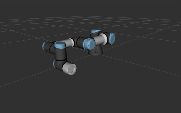
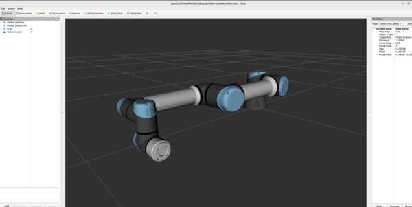
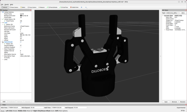
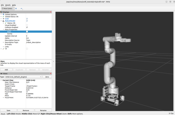
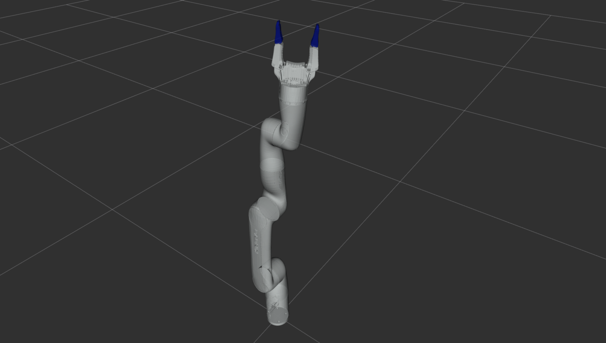
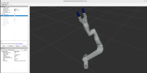
Let’s see the URDF files in RViz first.
All of this is a single command below.
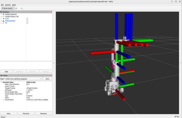
ros2 launch urdf_tutorial display.launch.py model:=/home/ubuntu/ros2_ws/src/kinova_robot_arm/kinova_robot_arm_description/urdf/gen3_lite_gen3_lite_2f.xacroUnder Global Options on the upper left panel of RViz, change the Fixed Frame from base_link to world.
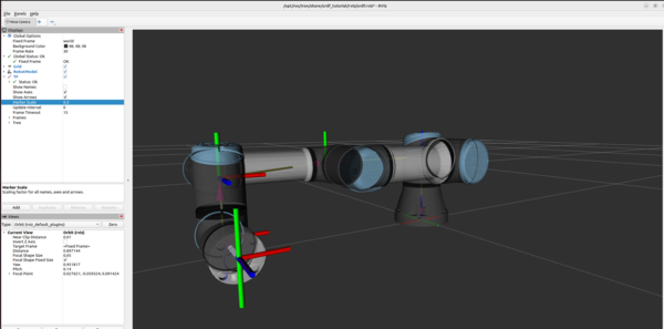
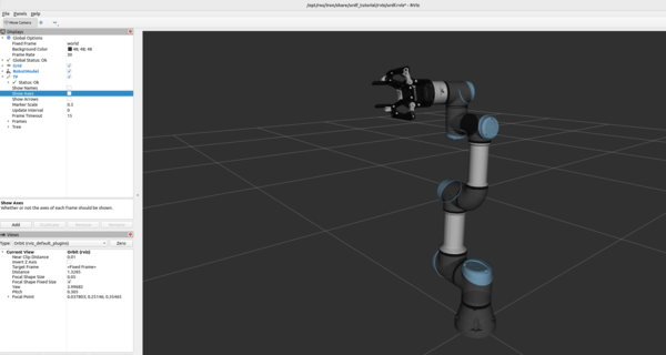
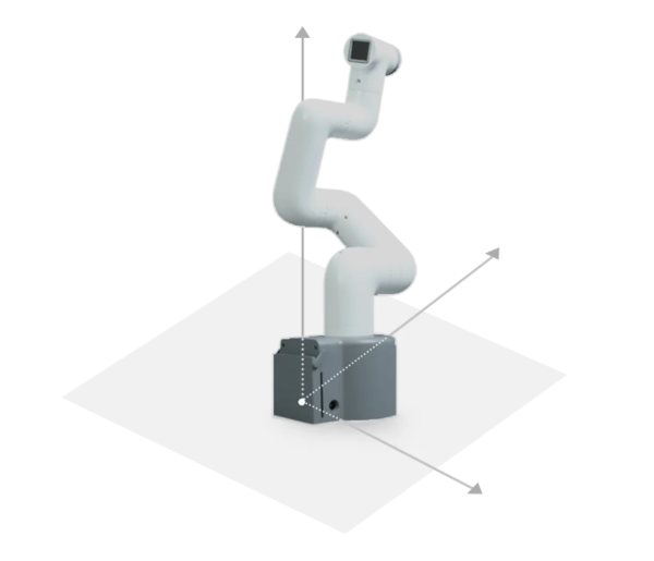
By convention, the red axis is the x-axis, the green axis in the y-axis, and the blue axis is the z-axis.
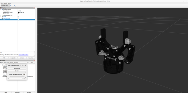
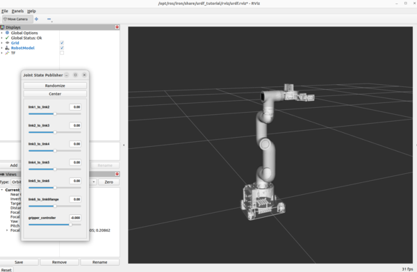
You can use the Joint State Publisher GUI pop-up window to move the links around.
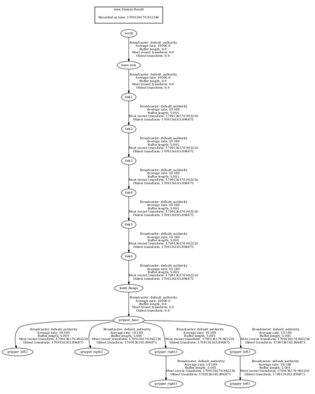
Open a new terminal window, and type the following command.
cd ~/Downloads/ros2 run tf2_tools view_framesTo see the coordinate frames, type:
evince your_file_name.pdfTo close RViz, press CTRL + C.