In this tutorial, we will learn about the Linear Quadratic Regulator (LQR). At the end, I’ll show you my example implementation of LQR in Python.

To get started, let’s take a look at what LQR is all about. Since LQR is an optimal feedback control technique, let’s start with the definition of optimal feedback control and then build our way up to LQR.

Real-World Applications

Here are a couple of real-world examples where you might find LQR control:

• Enabling a self-driving car to stay in the center of a lane or maintain a certain speed
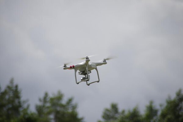
• Enabling a drone to hover at a specific altitude
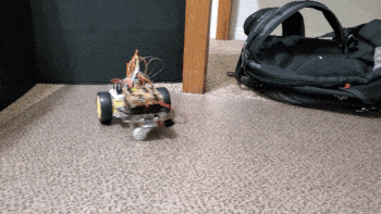
• Enabling a wheeled robot to follow a predetermined path

Prerequisites

• To understand this tutorial, it is helpful if you have completed my state space model tutorial.
• Otherwise, if you understand the concept of state space representation, jump right into this tutorial.

What is Optimal Feedback Control?

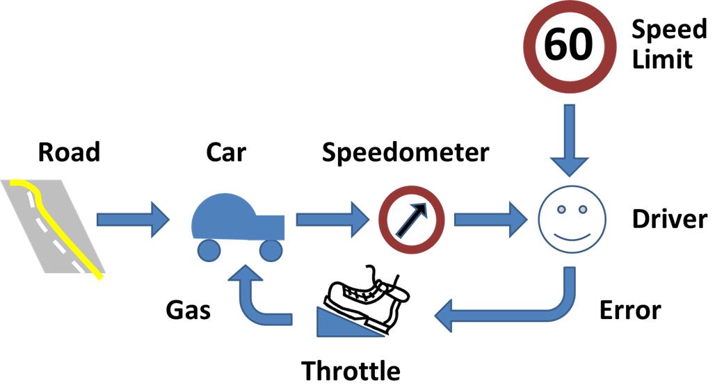
Consider these two real world examples:

• Example 1: You want a robot car to go from point A to point B along a predetermined path. 
• Example 2: You have a drone, and you want it to hover in the air at a specific altitude. You want it to take aerial photos of you. 

How do you accomplish both of these tasks?

Both the robot and the drone need to have a feedback control algorithm running inside them. 

The control algorithm’s job will be to output control signals (e.g. velocity of the wheels on the robot car, propeller speed, etc.) that reduce the error between the actual state (e.g. current position of the robot car or altitude for the drone) and the desired state. 

The sensors on the robot car/drone need to read the state of the system and feed that information back to the controller. 

The controller compares the actual state (i.e. the sensor information) with the desired state and then generates the best possible (i.e. optimal) control signals (often known as “system input”) that will reduce or eliminate that error.

In Example 1, the desired state is the (x,y) coordinate or GPS position along a predetermined path. At each timestep, you want the control algorithm to generate velocity commands for your robot that minimize the error between your current actual state (i.e. position) and the desired position (i.e. on top of the predetermined path).

In Example 2, with the drone, you want to minimize the error between your desired altitude of the drone and the actual altitude of the drone.

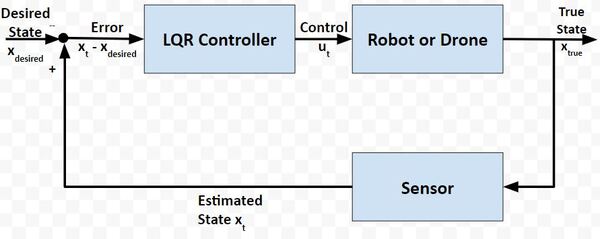
Here is how all that looks in a picture:

Your robot car and drone go through a continuous process of sensing the state of the system and then generating the best possible control commands to minimize the difference between the desired state x_desired and actual state x_t. 

The goal at each timestep (as the robot car drives along the path or the drone hovers in the air) is to use sensor feedback to drive the state error towards 0, where:

State error = x_t – x_desired

How Can We Drive State Error to 0 Efficiently?

Let’s revisit our examples from the previous section. 

Suppose in Example 2, a strong wind from a thunderstorm began to blow the drone downward, causing it to fall way below the desired altitude. 

To correct its altitude, the drone could:

• Action 1: Spin its propellers at top speed so that it shoots right up to the desired altitude as quickly as possible.
• Action 2: Gradually increase the speed of its propellers until it reaches the desired altitude.

Both Action 1 and 2 have pros and cons. 

Action 1

• Pros: Your drone returns to your desired altitude quickly. 
• Cons: Because the motors were spinning at top speed, you drained your drone’s battery significantly. Your drone now has only a few minutes of battery left before it dies, and the drone will soon come crashing down to Earth.

Action 2

• Pros: Less battery usage than Action 1
• Cons: It took seemingly forever for the drone to return to the desired altitude. 

How can we write a smart controller that balances both objectives? We want the system to both:

1. Have good control (i.e. stay on the desired path or altitude as closely as possible).
2. Minimize actuator (i.e. motor) effort as much as possible so the control inputs don’t cause the battery to drain so quickly. 

This, my friends, is where the Linear Quadratic Regulator (LQR) comes to the rescue. 

LQR Problem

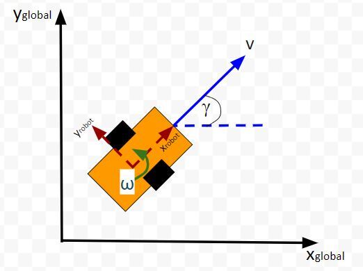
LQR solves a common problem when we’re trying to optimally control a robotic system. Going back to our robot car example, let’s draw its diagram. Here is our real world robot:

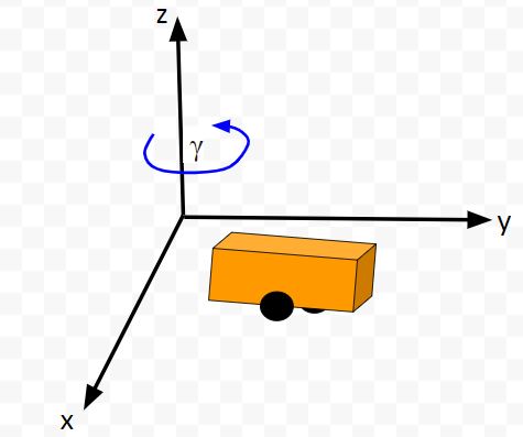
Let’s model this robot in a 3D diagram with coordinate axes x, y, and z:

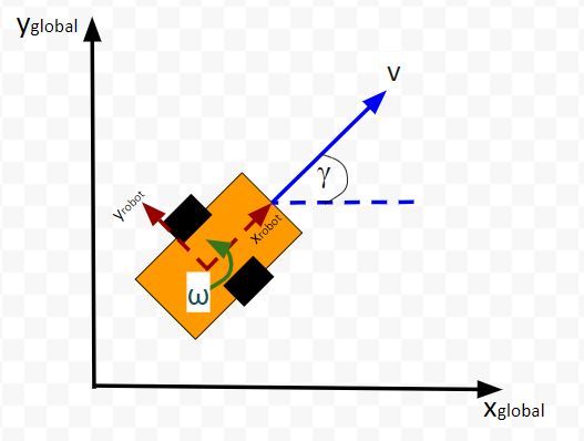
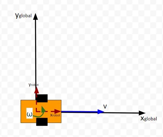
Here is the bird’s-eye view in 2D form:

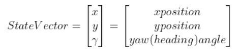
Suppose the robot car’s state at time t (position, orientation) is represented by vector x_t (e.g. where x_t = [x_global, y_global, orientation (yaw angle)].

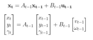
A state space model for this robotic system might look like the following:

where 

• x_t is the current state vector at time t in the global coordinate frame… [x_t, y_t,γ_t] = [x coordinate, y coordinate, yaw angle (i.e. rotation angle around the z-axis)]
• x_t-1 is the state vector at time t-1 in the global coordinate frame… [x_t-1, y_t-1,γ_t-1]
• u_t-1 represents the control input vector at time t-1… [v_t-1, ω_t-1] = [linear velocity, angular velocity]
• A and B are the state transition matrices.

(If that equation above doesn’t make a lot of sense, please check out the tutorial in the Prerequisites of this article where I dive into it in detail)

We want to choose control inputs u_t-1….such that

1. x_t actual – x_t desired is small…i.e. we get good control
2. u_t-1 is small…i.e. we use a minimal amount of actuator effort (i.e. control input, motor, etc.).

Both of these are competing objectives. A large u can drive the state error down really fast. A small u means the state error will remain really large. LQR was designed to solve this problem.

How LQR Works

The purpose of LQR is to compute the optimal control inputs u_t-1 (i.e. velocity of the wheels of a robotic car, motors for propellers of a drone) given:

1. Actual state x_t
2. Desired state x_t
3. State cost matrix Q (I’ll explain this term later in this tutorial)
4. Input cost matrix R (I’ll explain this term later in this tutorial) 
5. A matrix (See my state space modeling tutorial for how to calculate A)
6. B matrix (See my state space modeling tutorial for how to calculate B)
7. Time interval dt

that minimize the cumulative “cost.”

LQR is all about the cost function. It does some fancy math to come up with a function (this Wikipedia page shows the function) that expresses a “cost” (you could also substitute the word “penalty”) that is a function of both state error and actuator effort.

LQR’s goal is to minimize the “cost” of the state error, while minimizing the “cost” of actuator effort. 

• The higher the state error term, the higher the overall cost. 
• The higher the actuator effort term, the higher the overall cost. 

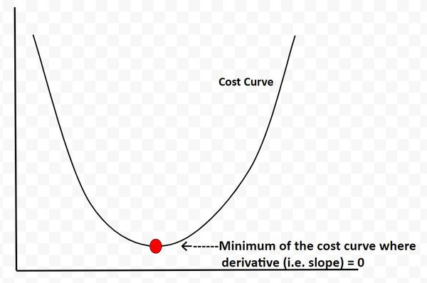
LQR determines the point along the cost curve where the “cost function” is minimized…thereby balancing both objectives of keeping state error and actuator effort minimized.

The cost curve below is for illustration purposes only. I’m using it just to explain this concept. In reality, the cost curve does not look like this. I’m using this graphic to convey to you the idea that LQR is all about finding the optimal control commands (i.e. linear velocity, angular velocity in the case of our robot car example) at which the actuator-effort state-error cost function is at a minimum. And from calculus, we know that the minimum of this cost function occurs at the point where the derivative (i.e. slope) is equal to 0.

We use some fancy math (I’ll get into this later) to find out what this point is.

What is Q?

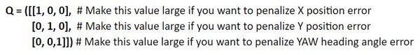
Q is called the state cost matrix. Q helps us weigh the relative importance of each state in the state vector (i.e. [x error,y error,yaw angle error]). 

Q is a square matrix that has the same number of rows and columns as there are states.

Q penalizes bad performance (e.g. penalizes large differences between where you want the robot to be vs. where it actually is in the world)

Q has positive values along the diagonal and zeros elsewhere.

Q enables us to target states where we want low error by making the corresponding value of Q large.

I typically start out with the identity matrix and then tweak the values through trial and error. In a 3-state system, such as with our two-wheeled robot car, Q would be the following 3×3 matrix:

What is R?

Similarly, R is the input cost matrix. This matrix penalizes actuator effort (i.e. rotation of the motors on the wheels). 

The R matrix has the same number of rows as are control inputs and the same number of columns as are control inputs. 

For example, imagine if we had a two-wheeled car with two control inputs, one for the linear velocity v and one for the angular velocity ω. 

The control input vector u_t-1 would be [linear velocity v in meters per second, angular velocity ω in radians per second].

The input cost matrix often has positive values along the diagonal. We can use this matrix to target actuator states where we want low actuator effort by making the corresponding value of R large.   

A lot of people start with the identity matrix, but I’ll start out with some low numbers. You want to tweak the values through trial and error.

In a case where we have two control inputs into a robotic system, here would be my starting 2×2 R matrix:

LQR Algorithm Pseudocode

LQR uses a technique called dynamic programming. You don’t need to worry what that means. 

At each timestep t as the robot or drone moves in the world, the optimal control input is calculated using a series of for loops (where we run each for loop ~N times) that spit out the u (i.e. control inputs) that corresponds to the minimal overall cost.

Here is the pseudocode for LQR. Hang tight. Go through this slowly. There is a lot of mathematical notation thrown around, and I want you to leave this tutorial with a solid understanding of LQR.

Let’s walk through this together. The pseudocode is in bold italics, and my comments are in plain text. You see below that the LQR function accepts 7 parameters.

LQR(Actual State x, Desired State xf, Q, R, A, B, dt):

x_error = Actual State x – Desired State xf

Initialize N = ## 

I typically set N to some arbitrary integer like 50. Solutions to LQR problems are obtained recursively, starting at the last time step, and working backwards in time to the first time step. 

In other words, the for loops (we’ll get to these in a second) need to go through lots of iterations (50 in this case) to reach a stable value for P (we’ll cover P in the next step).

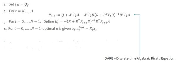
Set P = [Empty list of N + 1 elements]

Let P[N] = Q

For i = N, …, 1

P[i-1] = Q + A^TP[i]A – (A^TP[i]B)(R + B^TP[i]B)^-1(B^TP[i]A)   

This ugly equation above is called the Discrete-time Algebraic Riccati equation. Don’t be intimidated by it. You’ll notice that you have the values for all the terms on the right side of the equation. All that is required is plugging in values and computing the answer at each iteration step i so that you can fill in the list P.

K = [Empty list of N elements]

u = [Empty list of N elements]

For i = 0, …, N – 1

      K[i] = -(R + B^TP[i+1]B)^-1B^TP[i+1]A

K will hold the optimal feedback gain values. This is the important matrix that, when multiplied by the state error, will generate the optimal control inputs (see next step).

For i = 0, …, N – 1

      u[i] = K[i] @ x_error

We do N iterations of the for loop until we get a stable value for the optimal control input u (e.g. u = [linear velocity v, angular velocity ω]). I assume that a stable value is achieved when N=50.

u_star = u[N-1]  

Optimal control input is u_star. It is the last value we calculated in the previous step above. It is at the very end of the u list.

Return u_star  

Return the optimal control inputs. These inputs will be sent to our robot so that it can move to a new state (i.e. new x position, y position, and yaw angle γ).

Just for your future reference, you’ll commonly see the LQR algorithm written like this in the literature (and in college lectures):

LQR Python Code

Assumptions

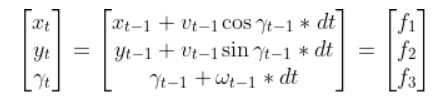
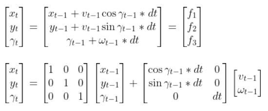
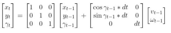
Let’s get back to our two-wheeled mobile robot. It has three states (like in the state space modeling tutorial.) The forward kinematics can be modeled as:

The state space model is as follows:

This model above shows the state of the robot at time t [x position, y position, yaw angle] given the state at time t-1, and the control inputs that were applied at time t-1.

The control inputs in this example are the linear velocity (v) — which has components in the x and y direction —  and the angular velocity around the z axis, ω (also known as the “yaw rate”).

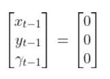
Our robot starts out at the origin (x=0 meters, y=0 meters), and the yaw angle is 0 radians. Thus the state at t-1 is:

We let dt = 1 second. dt represents the interval between timesteps.

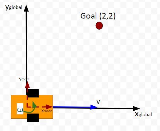
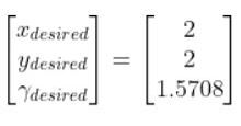
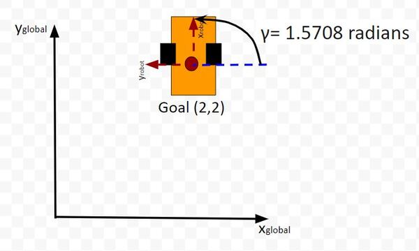
Now suppose we want our robot to drive to coordinate (x=2,y=2). This is our desired state (i.e. our goal destination).

Also, we want the robot to face due north (i.e. 90 degrees (1.5708 radians) yaw angle) once it reaches the desired state. Therefore, our desired state is:

We launch our robot at time t-1, and we feed it our desired state. The robot must use the LQR algorithm to solve for the optimal control inputs that minimize both the state error and actuator effort. In other words, we want the robot to get from (x=0, y=0) to (x=2, y=2) and face due north once we get there. However, we don’t want to get there so fast so that we drain the car’s battery.

These optimal control inputs then get fed into the control input vector to predict the state at time t.

In other words, we use LQR to solve for this:

And then plug that vector into this:

to get the state at time t.

One more thing to make this simulation more realistic. Let’s assume the maximum linear velocity of the robot car is 3.0 meters per second, and the maximum angular velocity is 90 degrees per second (1.5708 radians per second).

Let’s take a look at all this in Python code.

Code

Here is my Python implementation of the LQR. Don’t be intimidated by all the lines of code. Just go through it one step at a time. Take your time. You can copy and paste the entire thing into your favorite IDE.

Remember to play with the values along the diagonals of the Q and R matrices. You’ll see in my code that the Q matrix has been tweaked a bit.

import numpy as np

# Author: Addison Sears-Collins
# https://automaticaddison.com
# Description: Linear Quadratic Regulator example 
#	(two-wheeled differential drive robot car)

######################## DEFINE CONSTANTS #####################################
# Supress scientific notation when printing NumPy arrays
np.set_printoptions(precision=3,suppress=True)

# Optional Variables
max_linear_velocity = 3.0 # meters per second
max_angular_velocity = 1.5708 # radians per second

def getB(yaw, deltat):
	"""
	Calculates and returns the B matrix
	3x2 matix ---> number of states x number of control inputs

	Expresses how the state of the system [x,y,yaw] changes
	from t-1 to t due to the control commands (i.e. control inputs).
	
	:param yaw: The yaw angle (rotation angle around the z axis) in radians 
	:param deltat: The change in time from timestep t-1 to t in seconds
	
	:return: B matrix ---> 3x2 NumPy array
	"""
	B = np.array([	[np.cos(yaw)*deltat, 0],
									[np.sin(yaw)*deltat, 0],
									[0, deltat]])
	return B


def state_space_model(A, state_t_minus_1, B, control_input_t_minus_1):
	"""
	Calculates the state at time t given the state at time t-1 and
	the control inputs applied at time t-1
	
	:param: A	The A state transition matrix
		3x3 NumPy Array
	:param: state_t_minus_1 	The state at time t-1  
		3x1 NumPy Array given the state is [x,y,yaw angle] ---> 
		[meters, meters, radians]
	:param: B 	The B state transition matrix
		3x2 NumPy Array
	:param: control_input_t_minus_1 	Optimal control inputs at time t-1  
		2x1 NumPy Array given the control input vector is 
		[linear velocity of the car, angular velocity of the car]
		[meters per second, radians per second]
		
	:return: State estimate at time t
		3x1 NumPy Array given the state is [x,y,yaw angle] --->
		[meters, meters, radians]
	"""	
	# These next 6 lines of code which place limits on the angular and linear 
	# velocities of the robot car can be removed if you desire.
	control_input_t_minus_1[0] = np.clip(control_input_t_minus_1[0],
																			-max_linear_velocity,
																			max_linear_velocity)
	control_input_t_minus_1[1] = np.clip(control_input_t_minus_1[1],
																			-max_angular_velocity,
																			max_angular_velocity)
	state_estimate_t = (A @ state_t_minus_1) + (B @ control_input_t_minus_1) 
			
	return state_estimate_t
	
def lqr(actual_state_x, desired_state_xf, Q, R, A, B, dt):
	"""
	Discrete-time linear quadratic regulator for a nonlinear system.

	Compute the optimal control inputs given a nonlinear system, cost matrices, 
	current state, and a final state.
	
	Compute the control variables that minimize the cumulative cost.

	Solve for P using the dynamic programming method.

	:param actual_state_x: The current state of the system 
		3x1 NumPy Array given the state is [x,y,yaw angle] --->
		[meters, meters, radians]
	:param desired_state_xf: The desired state of the system
		3x1 NumPy Array given the state is [x,y,yaw angle] --->
		[meters, meters, radians]	
	:param Q: The state cost matrix
		3x3 NumPy Array
	:param R: The input cost matrix
		2x2 NumPy Array
	:param dt: The size of the timestep in seconds -> float

	:return: u_star: Optimal action u for the current state 
		2x1 NumPy Array given the control input vector is
		[linear velocity of the car, angular velocity of the car]
		[meters per second, radians per second]
    """
	# We want the system to stabilize at desired_state_xf.
	x_error = actual_state_x - desired_state_xf

	# Solutions to discrete LQR problems are obtained using the dynamic 
	# programming method.
	# The optimal solution is obtained recursively, starting at the last 
	# timestep and working backwards.
	# You can play with this number
	N = 50

	# Create a list of N + 1 elements
	P = [None] * (N + 1)
	
	Qf = Q

	# LQR via Dynamic Programming
	P[N] = Qf

	# For i = N, ..., 1
	for i in range(N, 0, -1):

		# Discrete-time Algebraic Riccati equation to calculate the optimal 
		# state cost matrix
		P[i-1] = Q + A.T @ P[i] @ A - (A.T @ P[i] @ B) @ np.linalg.pinv(
			R + B.T @ P[i] @ B) @ (B.T @ P[i] @ A)      

	# Create a list of N elements
	K = [None] * N
	u = [None] * N

	# For i = 0, ..., N - 1
	for i in range(N):

		# Calculate the optimal feedback gain K
		K[i] = -np.linalg.pinv(R + B.T @ P[i+1] @ B) @ B.T @ P[i+1] @ A

		u[i] = K[i] @ x_error

	# Optimal control input is u_star
	u_star = u[N-1]

	return u_star

def main():
	
	# Let the time interval be 1.0 seconds
	dt = 1.0
	
	# Actual state
	# Our robot starts out at the origin (x=0 meters, y=0 meters), and 
	# the yaw angle is 0 radians. 
	actual_state_x = np.array([0,0,0]) 

	# Desired state [x,y,yaw angle]
	# [meters, meters, radians]
	desired_state_xf = np.array([2.000,2.000,np.pi/2])	
	
	# A matrix
	# 3x3 matrix -> number of states x number of states matrix
	# Expresses how the state of the system [x,y,yaw] changes 
	# from t-1 to t when no control command is executed.
	# Typically a robot on wheels only drives when the wheels are told to turn.
	# For this case, A is the identity matrix.
	# Note: A is sometimes F in the literature.
	A = np.array([	[1.0,  0,   0],
									[  0,1.0,   0],
									[  0,  0, 1.0]])

	# R matrix
	# The control input cost matrix
	# Experiment with different R matrices
	# This matrix penalizes actuator effort (i.e. rotation of the 
	# motors on the wheels that drive the linear velocity and angular velocity).
	# The R matrix has the same number of rows as the number of control
	# inputs and same number of columns as the number of 
	# control inputs.
	# This matrix has positive values along the diagonal and 0s elsewhere.
	# We can target control inputs where we want low actuator effort 
	# by making the corresponding value of R large. 
	R = np.array([[0.01,   0],  # Penalty for linear velocity effort
                [  0, 0.01]]) # Penalty for angular velocity effort

	# Q matrix
	# The state cost matrix.
	# Experiment with different Q matrices.
	# Q helps us weigh the relative importance of each state in the 
	# state vector (X, Y, YAW ANGLE). 
	# Q is a square matrix that has the same number of rows as 
	# there are states.
	# Q penalizes bad performance.
	# Q has positive values along the diagonal and zeros elsewhere.
	# Q enables us to target states where we want low error by making the 
	# corresponding value of Q large.
	Q = np.array([[0.639, 0, 0],  # Penalize X position error 
								[0, 1.0, 0],  # Penalize Y position error 
								[0, 0, 1.0]]) # Penalize YAW ANGLE heading error 
				  
	# Launch the robot, and have it move to the desired goal destination
	for i in range(100):
		print(f'iteration = {i} seconds')
		print(f'Current State = {actual_state_x}')
		print(f'Desired State = {desired_state_xf}')
		
		state_error = actual_state_x - desired_state_xf
		state_error_magnitude = np.linalg.norm(state_error)		
		print(f'State Error Magnitude = {state_error_magnitude}')
		
		B = getB(actual_state_x[2], dt)
		
		# LQR returns the optimal control input
		optimal_control_input = lqr(actual_state_x, 
									desired_state_xf, 
									Q, R, A, B, dt)	
		
		print(f'Control Input = {optimal_control_input}')
									
		
		# We apply the optimal control to the robot
		# so we can get a new actual (estimated) state.
		actual_state_x = state_space_model(A, actual_state_x, B, 
										optimal_control_input)	

		# Stop as soon as we reach the goal
		# Feel free to change this threshold value.
		if state_error_magnitude < 0.01:
			print("\nGoal Has Been Reached Successfully!")
			break
			
		print()

# Entry point for the program
main()

Output

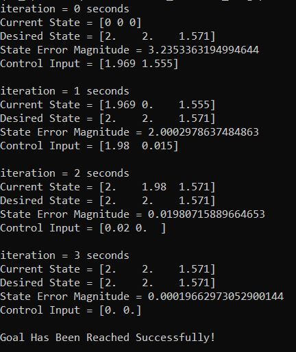
You can see in the output that it took about 3 seconds for the robot to reach the goal position and orientation. The LQR algorithm did its job well.

Note that you can remove the maximum linear and angular velocity constraints if you have issues in getting the correct output. You can remove these constraints by going to the state_space_model method inside the code I pasted in the previous section.

Conclusion

That’s it for the fundamentals of LQR. If you ever run across LQR in the future and need a refresher, just come back to this tutorial. 

Keep building!