If you want to use GPU support for your TensorFlow installation, you will need to follow these steps. If you have trouble following those steps, you can follow these steps (note that the steps change quite frequently, but the overall process remains relatively the same).
This post can also help you get your system setup, including your virtual environment in Anaconda (if you decide to go this route).
Helpful Tip
When you work through tutorials in robotics or any other field in technology, focus on the end goal. Focus on the authentic, real-world problem you’re trying to solve, not the tools that are used to solve the problem.
Don’t get bogged down in trying to understand every last detail of the math and the libraries you need to use to develop an application.
Don’t get stuck in rabbit holes. Don’t try to learn everything at once.
You’re trying to build products not publish research papers. Focus on the inputs, the outputs, and what the algorithm is supposed to do at a high level. As you’ll see in this tutorial, you don’t need to learn all of computer vision before developing a robust road sign classification system.
Get a working road sign detector and classifier up and running; and, at some later date when you want to add more complexity to your project or write a research paper, then feel free to go back to the rabbit holes to get a thorough understanding of what is going on under the hood.
Trying to understand every last detail is like trying to build your own database from scratch in order to start a website or taking a course on internal combustion engines to learn how to drive a car.
Let’s get started!
Find a Data Set
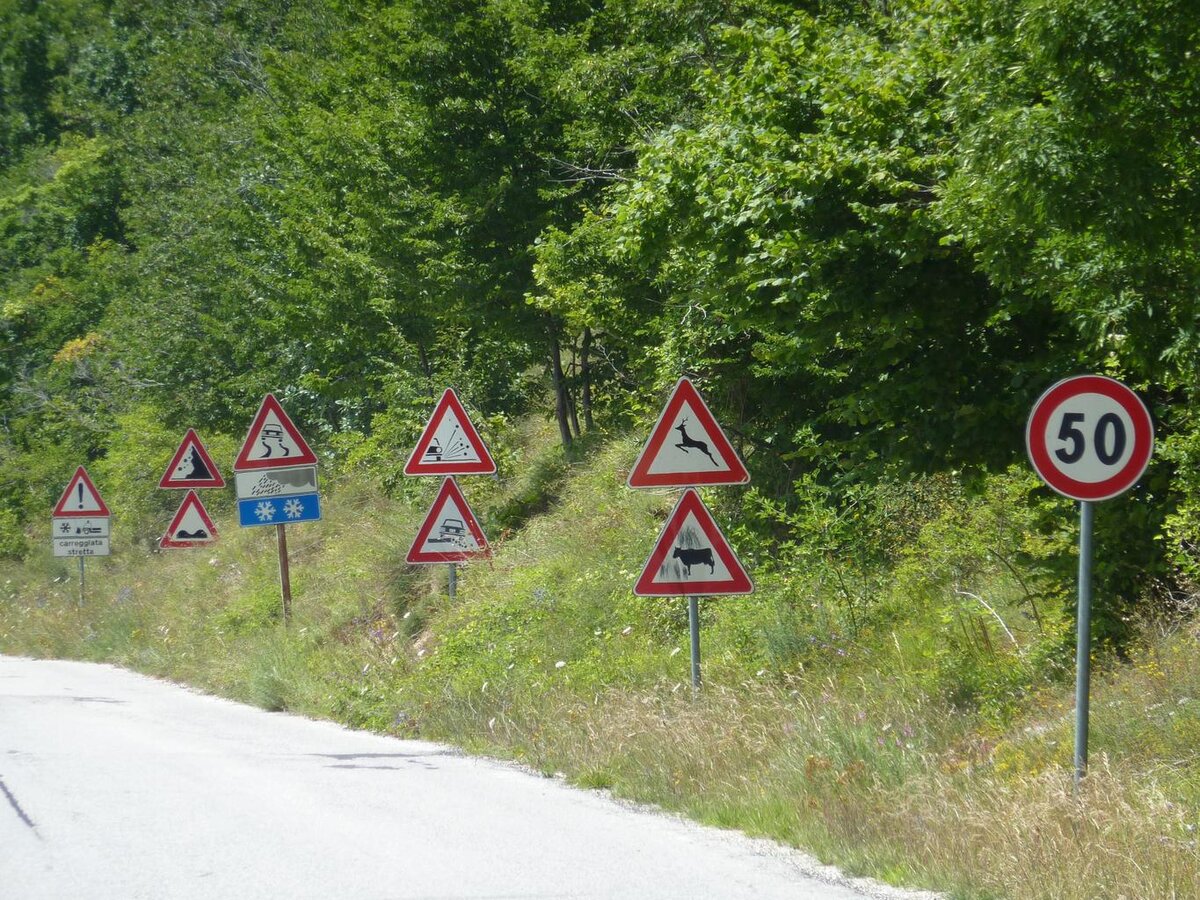
The first thing we need to do is find a data set of road signs.
We will use the popular German Traffic Sign Recognition Benchmark data set. This data set consists of more than 43 different road sign types and 50,000+ images. Each image contains a single traffic sign.
Download the Data Set
Go to this link, and download the data set. You will see three data files.
Training data set
Validation data set
Test data set
The data files are .p (pickle) files.
What is a pickle file? Pickling is where you convert a Python object (dictionary, list, etc.) into a stream of characters. That stream of characters is saved as a .p file. This process is known as serialization.
Then, when you want to use the Python object in another script, you can use the Pickle library to convert that stream of characters back to the original Python object. This process is known as deserialization.
Training, validation, and test data sets in computer vision can be large, so pickling them in order to save them to your computer reduces storage space.
Installation and Setup
We need to make sure we have all the software packages installed.
Make sure you have NumPy installed, a scientific computing library for Python.
If you’re using Anaconda, you can type:
conda install numpy
Alternatively, you can type:
pip install numpy
Install Matplotlib, a plotting library for Python.
For Anaconda users:
conda install -c conda-forge matplotlib
Otherwise, you can install like this:
pip install matplotlib
Install scikit-learn, the machine learning library:
conda install -c conda-forge scikit-learn
Write the Code
Open a new Python file called load_road_sign_data.py
Here is the full code for the road sign detection and classification system:
# Project: How to Detect and Classify Road Signs Using TensorFlow
# Author: Addison Sears-Collins
# Date created: February 13, 2021
# Description: This program loads the German Traffic Sign
# Recognition Benchmark data set
import warnings # Control warning messages that pop up
warnings.filterwarnings("ignore") # Ignore all warnings
import matplotlib.pyplot as plt # Plotting library
import matplotlib.image as mpimg
import numpy as np # Scientific computing library
import pandas as pd # Library for data analysis
import pickle # Converts an object into a character stream (i.e. serialization)
import random # Pseudo-random number generator library
from sklearn.model_selection import train_test_split # Split data into subsets
from sklearn.utils import shuffle # Machine learning library
from subprocess import check_output # Enables you to run a subprocess
import tensorflow as tf # Machine learning library
from tensorflow import keras # Deep learning library
from tensorflow.keras import layers # Handles layers in the neural network
from tensorflow.keras.models import load_model # Loads a trained neural network
from tensorflow.keras.utils import plot_model # Get neural network architecture
# Open the training, validation, and test data sets
with open("./road-sign-data/train.p", mode='rb') as training_data:
train = pickle.load(training_data)
with open("./road-sign-data/valid.p", mode='rb') as validation_data:
valid = pickle.load(validation_data)
with open("./road-sign-data/test.p", mode='rb') as testing_data:
test = pickle.load(testing_data)
# Store the features and the labels
X_train, y_train = train['features'], train['labels']
X_valid, y_valid = valid['features'], valid['labels']
X_test, y_test = test['features'], test['labels']
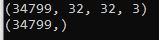
# Output the dimensions of the training data set
# Feel free to uncomment these lines below
#print(X_train.shape)
#print(y_train.shape)
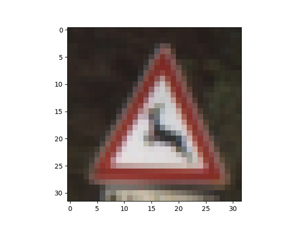
# Display an image from the data set
i = 500
#plt.imshow(X_train[i])
#plt.show() # Uncomment this line to display the image
#print(y_train[i])
# Shuffle the image data set
X_train, y_train = shuffle(X_train, y_train)
# Convert the RGB image data set into grayscale
X_train_grscale = np.sum(X_train/3, axis=3, keepdims=True)
X_test_grscale = np.sum(X_test/3, axis=3, keepdims=True)
X_valid_grscale = np.sum(X_valid/3, axis=3, keepdims=True)
# Normalize the data set
# Note that grayscale has a range from 0 to 255 with 0 being black and
# 255 being white
X_train_grscale_norm = (X_train_grscale - 128)/128
X_test_grscale_norm = (X_test_grscale - 128)/128
X_valid_grscale_norm = (X_valid_grscale - 128)/128
# Display the shape of the grayscale training data
#print(X_train_grscale.shape)
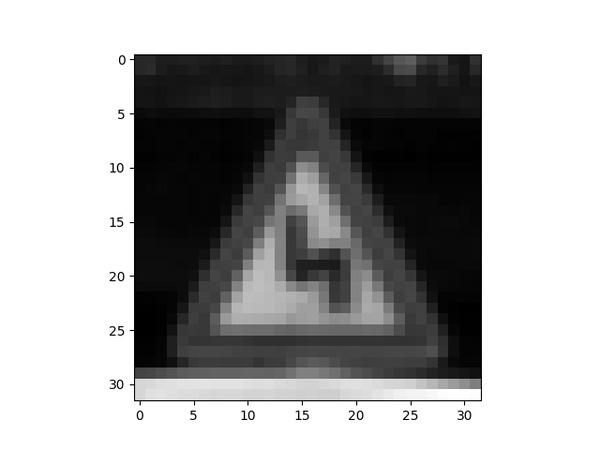
# Display a sample image from the grayscale data set
i = 500
# squeeze function removes axes of length 1
# (e.g. arrays like [[[1,2,3]]] become [1,2,3])
#plt.imshow(X_train_grscale[i].squeeze(), cmap='gray')
#plt.figure()
#plt.imshow(X_train[i])
#plt.show()
# Get the shape of the image
# IMG_SIZE, IMG_SIZE, IMG_CHANNELS
img_shape = X_train_grscale[i].shape
#print(img_shape)
# Build the convolutional neural network's (i.e. model) architecture
cnn_model = tf.keras.Sequential() # Plain stack of layers
cnn_model.add(tf.keras.layers.Conv2D(filters=32,kernel_size=(3,3),
strides=(3,3), input_shape = img_shape, activation='relu'))
cnn_model.add(tf.keras.layers.Conv2D(filters=64,kernel_size=(3,3),
activation='relu'))
cnn_model.add(tf.keras.layers.MaxPooling2D(pool_size = (2, 2)))
cnn_model.add(tf.keras.layers.Dropout(0.25))
cnn_model.add(tf.keras.layers.Flatten())
cnn_model.add(tf.keras.layers.Dense(128, activation='relu'))
cnn_model.add(tf.keras.layers.Dropout(0.5))
cnn_model.add(tf.keras.layers.Dense(43, activation = 'sigmoid')) # 43 classes
# Compile the model
cnn_model.compile(loss='sparse_categorical_crossentropy', optimizer=(
keras.optimizers.Adam(
0.001, beta_1=0.9, beta_2=0.999, epsilon=1e-07, amsgrad=False)), metrics =[
'accuracy'])
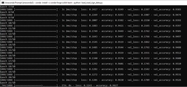
# Train the model
history = cnn_model.fit(x=X_train_grscale_norm,
y=y_train,
batch_size=32,
epochs=50,
verbose=1,
validation_data = (X_valid_grscale_norm,y_valid))
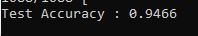
# Show the loss value and metrics for the model on the test data set
score = cnn_model.evaluate(X_test_grscale_norm, y_test,verbose=0)
print('Test Accuracy : {:.4f}'.format(score[1]))
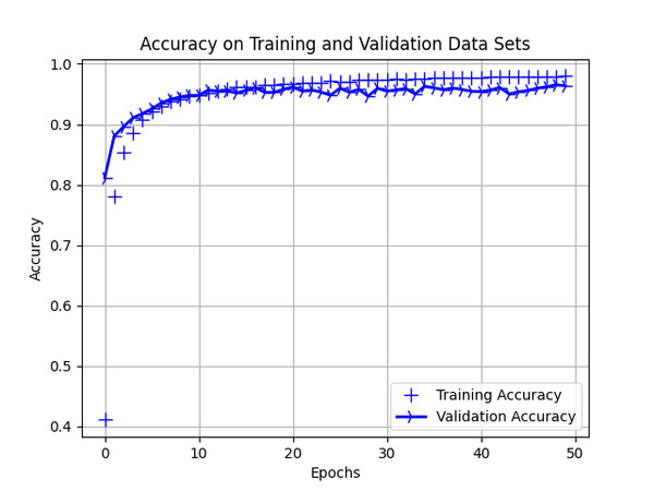
# Plot the accuracy statistics of the model on the training and valiation data
accuracy = history.history['accuracy']
val_accuracy = history.history['val_accuracy']
epochs = range(len(accuracy))
## Uncomment these lines below to show accuracy statistics
# line_1 = plt.plot(epochs, accuracy, 'bo', label='Training Accuracy')
# line_2 = plt.plot(epochs, val_accuracy, 'b', label='Validation Accuracy')
# plt.title('Accuracy on Training and Validation Data Sets')
# plt.setp(line_1, linewidth=2.0, marker = '+', markersize=10.0)
# plt.setp(line_2, linewidth=2.0, marker= '4', markersize=10.0)
# plt.xlabel('Epochs')
# plt.ylabel('Accuracy')
# plt.grid(True)
# plt.legend()
# plt.show() # Uncomment this line to display the plot
# Save the model
cnn_model.save("./road_sign.h5")
# Reload the model
model = load_model('./road_sign.h5')
# Get the predictions for the test data set
predicted_classes = np.argmax(cnn_model.predict(X_test_grscale_norm), axis=-1)
# Retrieve the indices that we will plot
y_true = y_test
# Plot some of the predictions on the test data set
for i in range(15):
plt.subplot(5,3,i+1)
plt.imshow(X_test_grscale_norm[i].squeeze(),
cmap='gray', interpolation='none')
plt.title("Predict {}, Actual {}".format(predicted_classes[i],
y_true[i]), fontsize=10)
plt.tight_layout()
plt.savefig('road_sign_output.png')
plt.show()
How the Code Works
Let’s go through each snippet of code in the previous section so that we understand what is going on.
Load the Image Data
The first thing we need to do is to load the image data from the pickle files.
with open("./road-sign-data/train.p", mode='rb') as training_data:
  train = pickle.load(training_data)
with open("./road-sign-data/valid.p", mode='rb') as validation_data:
  valid = pickle.load(validation_data)
with open("./road-sign-data/test.p", mode='rb') as testing_data:
  test = pickle.load(testing_data)
accuracy = history.history['accuracy']
val_accuracy = history.history['val_accuracy']
epochs = range(len(accuracy))

line_1 = plt.plot(epochs, accuracy, 'bo', label='Training Accuracy')
line_2 = plt.plot(epochs, val_accuracy, 'b', label='Validation Accuracy')
plt.title('Accuracy on Training and Validation Data Sets')
plt.setp(line_1, linewidth=2.0, marker = '+', markersize=10.0)
plt.setp(line_2, linewidth=2.0, marker= '4', markersize=10.0)
plt.xlabel('Epochs')
plt.ylabel('Accuracy')
plt.grid(True)
plt.legend()
plt.show() # Uncomment this line to display the plot
Save the Convolutional Neural Network to a File
We save the trained neural network so that we can use it in another application at a later date.
cnn_model.save("./road_sign.h5")
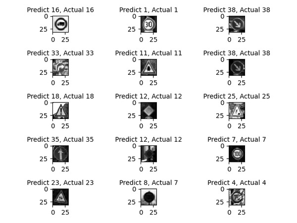
Verify the Output
Finally, we take a look at some of the output to see how our neural network performs on unseen data. You can see in this subset that the neural network correctly classified 14 out of the 15 test examples.
# Reload the model
model = load_model('./road_sign.h5')

# Get the predictions for the test data set
predicted_classes = np.argmax(cnn_model.predict(X_test_grscale_norm), axis=-1)

# Retrieve the indices that we will plot
y_true = y_test

# Plot some of the predictions on the test data set
for i in range(15):
  plt.subplot(5,3,i+1)
  plt.imshow(X_test_grscale_norm[i].squeeze(),
    cmap='gray', interpolation='none')
  plt.title("Predict {}, Actual {}".format(predicted_classes[i],
    y_true[i]), fontsize=10)
plt.tight_layout()
plt.savefig('road_sign_output.png')
plt.show()
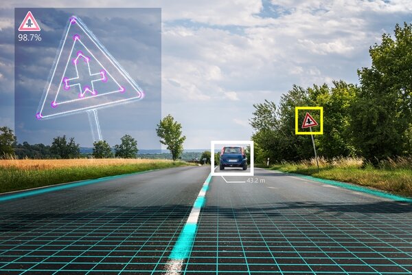
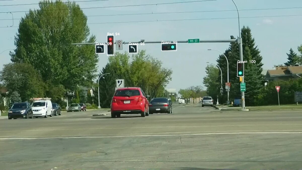
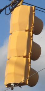
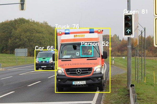
In this tutorial, we will develop a program to detect traffic lights and then classify their color (e.g. red, green, and yellow). Our program will first use a pretrained neural network to detect traffic lights, then it will run those detections through another neural network which is trained to identify the color. By the end of this tutorial, you will be able to develop this:
Our goal is to build an early prototype of a system that can be used in an autonomous vehicle.
If you want to use GPU support for your TensorFlow installation, you will need to follow these steps. If you have trouble following those steps, you can follow these steps (note that the steps change quite frequently, but the overall process remains relatively the same).
This post can also help you get your system setup, including your virtual environment in Anaconda (if you decide to go this route).
This tutorial is not a prerequisite, but it is one of the best tutorials on the Internet for the step-by-step process of how to detect objects in an image or a video using Tensorflow 2.
Helpful Tip
As you work through this tutorial, focus on the end goals I listed in the beginning. Don’t get bogged down in trying to understand every last detail of the math and the libraries we will use to develop the application.
We are trying to build products not publish research papers. Focus on the inputs, the outputs, and what the algorithm is supposed to do at a high level.
Get a working traffic light detector and classifier up and running; and, at some later date when you want to add more complexity to your project or write a research paper, you can dive deeper under the hood to understand all the details.
Trying to understand every last detail is like trying to build your own database from scratch in order to start a website or taking a course on internal combustion engines to learn how to drive a car.
Let’s get started!
Find Some Videos and an Image
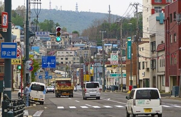
The first thing we need to do is find some videos and an image to serve as our test cases.
We want to download videos and images that show traffic lights. Images of streets from the point of view of a driver in a car are good candidates.
I found some good candidates on Pixabay.com and Dreamstime.com. Type “driving” or “traffic lights” in the video search on that website.
We now need to make sure we have all the software packages installed. Check to see if you have OpenCV installed on your machine. If you are using Anaconda, you can type:
conda install -c conda-forge opencv
Alternatively, you can type:
pip install opencv-python
Make sure you have NumPy installed, a scientific computing library for Python.
If you’re using Anaconda, you can type:
conda install numpy
Alternatively, you can type:
pip install numpy
Install Matplotlib, a plotting library for Python.
For Anaconda users:
conda install -c conda-forge matplotlib
Otherwise, you can install like this:
pip install matplotlib
Extract Traffic Lights From Images
We now need to go through all of our images and extract the traffic lights. We want a good mix of green, yellow, and red traffic light examples.
To do this, we will create two programs:
extract_traffic_lights.py: This program is the driver. You will run this program to create cropped images of traffic lights.
object_detection.py: This program contains a bunch of methods for traffic light detection (as well as other objects like pedestrians, cars, and stop signs).
Here is the code for extract_traffic_lights.py:
# Project: How to Detect and Classify Traffic Lights
# Author: Addison Sears-Collins
# Date created: January 11, 2021
# Description: This program extracts traffic lights from images.

import cv2 # Computer vision library
import object_detection # Contains methods for object detection in images

# Get a list of jpeg image files containing traffic lights
files = object_detection.get_files('traffic_light_input/*.jpg')

# Load the object detection model
this_model = object_detection.load_ssd_coco()

# Keep track of the number of traffic lights found
traffic_light_count = 0

# Keep track of the number of image files that were processed
file_count = 0

# Display a count of the number of images we need to process
print("Number of Images:", len(files))

# Go through each image file, one at a time
for file in files:

  # Detect objects in the image
  # img_rgb is the original image in RGB format
  # out is a dictionary containing the results of object detection
  # file_name is the name of the file
  (img_rgb, out, file_name) = object_detection.perform_object_detection(model=this_model, file_name=file, save_annotated=None, model_traffic_lights=None)

  # Every 10 files that are processed
  if (file_count % 10) == 0:

    # Display a count of the number of files that have been processed
    print("Images processed:", file_count)

    # Display the total number of traffic lights that have been identified so far
    print("Number of Traffic lights identified: ", traffic_light_count)

  # Increment the number of files by 1
  file_count = file_count + 1

  # For each traffic light (i.e. bounding box) that was detected
  for idx in range(len(out['boxes'])):

    # Extract the type of object that was detected
    obj_class = out["detection_classes"][idx]

    # If the object that was detected is a traffic light
    if obj_class == object_detection.LABEL_TRAFFIC_LIGHT:

      # Extract the coordinates of the bounding box
      box = out["boxes"][idx]

      # Extract (i.e. crop) the traffic light from the image
      traffic_light = img_rgb[box["y"]:box["y2"], box["x"]:box["x2"]]

      # Convert the traffic light from RGB format into BGR format
      traffic_light = cv2.cvtColor(traffic_light, cv2.COLOR_RGB2BGR)

      # Store the cropped image in a folder named 'traffic_light_cropped'
      cv2.imwrite("traffic_light_cropped/" + str(traffic_light_count) + ".jpg", traffic_light)

      # Increment the number of traffic lights by 1
      traffic_light_count = traffic_light_count + 1

# Display the total number of traffic lights identified
print("Number of Traffic lights identified:", traffic_light_count)
Here is the code for object_detection.py:
# Project: How to Detect and Classify Traffic Lights
# Author: Addison Sears-Collins
# Date created: January 11, 2021
# Description: This program helps detect objects (e.g. traffic lights) in
#   images.

import tensorflow as tf # Machine learning library
from tensorflow import keras # Library for neural networks
import numpy as np # Scientific computing library
import cv2 # Computer vision library
import glob # Filename handling library

# Inception V3 model for Keras
from tensorflow.keras.applications.inception_v3 import preprocess_input

# To detect objects, we will use a pretrained neural network that has been
# trained on the COCO data set. You can read more about this data set here:
#   https://content.alegion.com/datasets/coco-ms-coco-dataset
# COCO labels are here: https://github.com/tensorflow/models/blob/master/research/object_detection/data/mscoco_label_map.pbtxt
LABEL_PERSON = 1
LABEL_CAR = 3
LABEL_BUS = 6
LABEL_TRUCK = 8
LABEL_TRAFFIC_LIGHT = 10
LABEL_STOP_SIGN = 13

def accept_box(boxes, box_index, tolerance):
  """
  Eliminate duplicate bounding boxes.
  """
  box = boxes[box_index]

  for idx in range(box_index):
    other_box = boxes[idx]
    if abs(center(other_box, "x") - center(box, "x")) < tolerance and abs(center(other_box, "y") - center(box, "y")) < tolerance:
      return False

  return True

def get_files(pattern):
  """
  Create a list of all the images in a directory

  :param:pattern str The pattern of the filenames
  :return: A list of the files that match the specified pattern
  """
  files = []

  # For each file that matches the specified pattern
  for file_name in glob.iglob(pattern, recursive=True):

    # Add the image file to the list of files
    files.append(file_name)

  # Return the complete file list
  return files

def load_model(model_name):
  """
  Download a pretrained object detection model, and save it to your hard drive.
  :param:str Name of the pretrained object detection model
  """
  url = 'http://download.tensorflow.org/models/object_detection/tf2/20200711/' + model_name + '.tar.gz'

  # Download a file from a URL that is not already in the cache
  model_dir = tf.keras.utils.get_file(fname=model_name, untar=True, origin=url)

  print("Model path: ", str(model_dir))

  model_dir = str(model_dir) + "/saved_model"
  model = tf.saved_model.load(str(model_dir))

  return model

def load_rgb_images(pattern, shape=None):
  """
  Loads the images in RGB format.

  :param:pattern str The pattern of the filenames
  :param:shape Image dimensions (width, height)
  """
  # Get a list of all the image files in a directory
  files = get_files(pattern)

  # For each image in the directory, convert it from BGR format to RGB format
  images = [cv2.cvtColor(cv2.imread(file), cv2.COLOR_BGR2RGB) for file in files]

  # Resize the image if the desired shape is provided
  if shape:
    return [cv2.resize(img, shape) for img in images]
  else:
    return images

def load_ssd_coco():
  """
  Load the neural network that has the SSD architecture, trained on the COCO
  data set.
  """
  return load_model("ssd_resnet50_v1_fpn_640x640_coco17_tpu-8")

def save_image_annotated(img_rgb, file_name, output, model_traffic_lights=None):
  """
  Annotate the image with the object types, and generate cropped images of
  traffic lights.
  """
  # Create annotated image file
  output_file = file_name.replace('.jpg', '_test.jpg')

  # For each bounding box that was detected
  for idx in range(len(output['boxes'])):

    # Extract the type of the object that was detected
    obj_class = output["detection_classes"][idx]

    # How confident the object detection model is on the object's type
    score = int(output["detection_scores"][idx] * 100)

    # Extract the bounding box
    box = output["boxes"][idx]

    color = None
    label_text = ""

    if obj_class == LABEL_PERSON:
      color = (0, 255, 255)
      label_text = "Person " + str(score)
    if obj_class == LABEL_CAR:
      color = (255, 255, 0)
      label_text = "Car " + str(score)
    if obj_class == LABEL_BUS:
      color = (255, 255, 0)
      label_text = "Bus " + str(score)
    if obj_class == LABEL_TRUCK:
      color = (255, 255, 0)
      label_text = "Truck " + str(score)
    if obj_class == LABEL_STOP_SIGN:
      color = (128, 0, 0)
      label_text = "Stop Sign " + str(score)
    if obj_class == LABEL_TRAFFIC_LIGHT:
      color = (255, 255, 255)
      label_text = "Traffic Light " + str(score)

      if model_traffic_lights:

			  # Annotate the image and save it
        img_traffic_light = img_rgb[box["y"]:box["y2"], box["x"]:box["x2"]]
        img_inception = cv2.resize(img_traffic_light, (299, 299))

				# Uncomment this if you want to save a cropped image of the traffic light
        #cv2.imwrite(output_file.replace('.jpg', '_crop.jpg'), cv2.cvtColor(img_inception, cv2.COLOR_RGB2BGR))
        img_inception = np.array([preprocess_input(img_inception)])

        prediction = model_traffic_lights.predict(img_inception)
        label = np.argmax(prediction)
        score_light = str(int(np.max(prediction) * 100))
        if label == 0:
          label_text = "Green " + score_light
        elif label == 1:
          label_text = "Yellow " + score_light
        elif label == 2:
          label_text = "Red " + score_light
        else:
          label_text = 'NO-LIGHT'  # This is not a traffic light

    if color and label_text and accept_box(output["boxes"], idx, 5.0) and score > 50:
      cv2.rectangle(img_rgb, (box["x"], box["y"]), (box["x2"], box["y2"]), color, 2)
      cv2.putText(img_rgb, label_text, (box["x"], box["y"]), cv2.FONT_HERSHEY_SIMPLEX, 0.7, (255, 255, 255), 2)

  cv2.imwrite(output_file, cv2.cvtColor(img_rgb, cv2.COLOR_RGB2BGR))
  print(output_file)

def center(box, coord_type):
  """
  Get center of the bounding box.
  """
  return (box[coord_type] + box[coord_type + "2"]) / 2

def perform_object_detection(model, file_name, save_annotated=False, model_traffic_lights=None):
  """
  Perform object detection on an image using the predefined neural network.
  """
  # Store the image
  img_bgr = cv2.imread(file_name)
  img_rgb = cv2.cvtColor(img_bgr, cv2.COLOR_BGR2RGB)
  input_tensor = tf.convert_to_tensor(img_rgb) # Input needs to be a tensor
  input_tensor = input_tensor[tf.newaxis, ...]

  # Run the model
  output = model(input_tensor)

  print("num_detections:", output['num_detections'], int(output['num_detections']))

  # Convert the tensors to a NumPy array
  num_detections = int(output.pop('num_detections'))
  output = {key: value[0, :num_detections].numpy()
            for key, value in output.items()}
  output['num_detections'] = num_detections

  print('Detection classes:', output['detection_classes'])
  print('Detection Boxes:', output['detection_boxes'])

  # The detected classes need to be integers.
  output['detection_classes'] = output['detection_classes'].astype(np.int64)
  output['boxes'] = [
    {"y": int(box[0] * img_rgb.shape[0]), "x": int(box[1] * img_rgb.shape[1]), "y2": int(box[2] * img_rgb.shape[0]),
     "x2": int(box[3] * img_rgb.shape[1])} for box in output['detection_boxes']]

  if save_annotated:
    save_image_annotated(img_rgb, file_name, output, model_traffic_lights)

  return img_rgb, output, file_name

def perform_object_detection_video(model, video_frame, model_traffic_lights=None):
  """
  Perform object detection on a video using the predefined neural network.

  Returns the annotated video frame.
  """
  # Store the image
  img_rgb = cv2.cvtColor(video_frame, cv2.COLOR_BGR2RGB)
  input_tensor = tf.convert_to_tensor(img_rgb) # Input needs to be a tensor
  input_tensor = input_tensor[tf.newaxis, ...]

  # Run the model
  output = model(input_tensor)

  # Convert the tensors to a NumPy array
  num_detections = int(output.pop('num_detections'))
  output = {key: value[0, :num_detections].numpy()
            for key, value in output.items()}
  output['num_detections'] = num_detections

  # The detected classes need to be integers.
  output['detection_classes'] = output['detection_classes'].astype(np.int64)
  output['boxes'] = [
    {"y": int(box[0] * img_rgb.shape[0]), "x": int(box[1] * img_rgb.shape[1]), "y2": int(box[2] * img_rgb.shape[0]),
     "x2": int(box[3] * img_rgb.shape[1])} for box in output['detection_boxes']]

  # For each bounding box that was detected
  for idx in range(len(output['boxes'])):

    # Extract the type of the object that was detected
    obj_class = output["detection_classes"][idx]

    # How confident the object detection model is on the object's type
    score = int(output["detection_scores"][idx] * 100)

    # Extract the bounding box
    box = output["boxes"][idx]

    color = None
    label_text = ""

    # if obj_class == LABEL_PERSON:
      # color = (0, 255, 255)
      # label_text = "Person " + str(score)
    # if obj_class == LABEL_CAR:
      # color = (255, 255, 0)
      # label_text = "Car " + str(score)
    # if obj_class == LABEL_BUS:
      # color = (255, 255, 0)
      # label_text = "Bus " + str(score)
    # if obj_class == LABEL_TRUCK:
      # color = (255, 255, 0)
      # label_text = "Truck " + str(score)
    if obj_class == LABEL_STOP_SIGN:
      color = (128, 0, 0)
      label_text = "Stop Sign " + str(score)
    if obj_class == LABEL_TRAFFIC_LIGHT:
      color = (255, 255, 255)
      label_text = "Traffic Light " + str(score)

      if model_traffic_lights:

			  # Annotate the image and save it
        img_traffic_light = img_rgb[box["y"]:box["y2"], box["x"]:box["x2"]]
        img_inception = cv2.resize(img_traffic_light, (299, 299))

        img_inception = np.array([preprocess_input(img_inception)])

        prediction = model_traffic_lights.predict(img_inception)
        label = np.argmax(prediction)
        score_light = str(int(np.max(prediction) * 100))
        if label == 0:
          label_text = "Green " + score_light
        elif label == 1:
          label_text = "Yellow " + score_light
        elif label == 2:
          label_text = "Red " + score_light
        else:
          label_text = 'NO-LIGHT'  # This is not a traffic light

    # Use the score variable to indicate how confident we are it is a traffic light (in % terms)
    # On the actual video frame, we display the confidence that the light is either red, green,
    # yellow, or not a valid traffic light.
    if color and label_text and accept_box(output["boxes"], idx, 5.0) and score > 20:
      cv2.rectangle(img_rgb, (box["x"], box["y"]), (box["x2"], box["y2"]), color, 2)
      cv2.putText(img_rgb, label_text, (box["x"], box["y"]), cv2.FONT_HERSHEY_SIMPLEX, 0.7, (255, 255, 255), 2)

  output_frame = cv2.cvtColor(img_rgb, cv2.COLOR_RGB2BGR)
  return output_frame

def double_shuffle(images, labels):
  """
  Shuffle the images to add some randomness.
  """
  indexes = np.random.permutation(len(images))

  return [images[idx] for idx in indexes], [labels[idx] for idx in indexes]

def reverse_preprocess_inception(img_preprocessed):
  """
  Reverse the preprocessing process.
  """
  img = img_preprocessed + 1.0
  img = img * 127.5
  return img.astype(np.uint8)
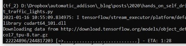
In order to detect the traffic lights in the image, we will use a pretrained object detection model available from TensorFlow. This model has been trained using the COCO data set.
When the model downloads, it will go to the C:\…\…\.keras\datasets folder. The first time you run extract_traffic_lights.py, the model will download to that directory.
Now, let’s run the program.
python extract_traffic_lights.py
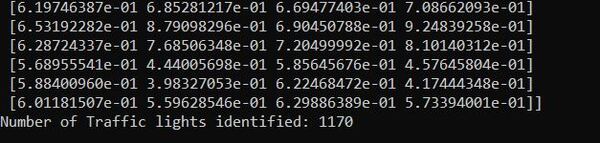
Here is what you should see when you run it.
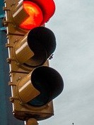
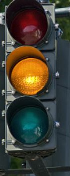
When you run the program above, it will generate a bunch of cropped images of traffic lights and save them inside the current directory in the traffic_light_cropped folder.
I had 1,170 cropped images of traffic lights (or pieces of traffic lights).
Here is what some of the cropped images look like:
Separate the Traffic Light Images by Color
We now need to separate the cropped images of traffic lights by color.
Create a new folder inside the current directory named traffic_light_dataset.
Inside the traffic_light_dataset folder, create three separate folders:
0_green
1_yellow
2_red
3_not
Go back to the traffic_light_cropped folder.
Grab some good images of green traffic lights, and place them in the 0_green folder.
Grab some good images of yellow traffic lights, and place them in the 1_yellow folder.
Grab some good images of red traffic lights, and place them in the 2_red folder.
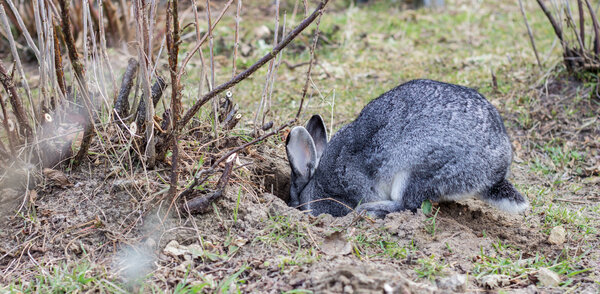
Grab some good images of the back and side of a traffic light (or pieces of buildings or something else that isn’t a traffic light), and place them in the 3_not folder. These images are your negative samples. Sometimes your neural network will classify an object as a traffic light, but it will actually be the back or side of a traffic light, so it isn’t useful for a self-driving car.
Here is an example of a 3_not image:
Note that the images are different sizes. This is exactly what we want.
We now have a custom traffic light data set that will enable us to train a neural network to detect the color of a traffic light.
The more images you have, the better. The performance of neural networks tends to improve with more training examples.
Use Transfer Learning to Create a Traffic Light Color Detection System
We are now going to use a technique called transfer learning to create a traffic light color detection system.
Transfer learning involves storing the knowledge gained while solving one problem and reapplying that knowledge to solve another, similar problem.
Within the same directory that contains the object_detection.py program, open up a new Python program called train_traffic_light_color.py. This program will train a neural network to detect traffic light color. The best neural network will be saved as traffic.h5.
20% of the images in the traffic_light_dataset folder will be the validation data set, and 80% of the images will be the training data set. The validation data set is used to tune the architecture of the neural network. It helps us to find the best neural network architecture to solve the problem (i.e. to determine the traffic light color).
The validation data set is also used to determine when the neural network needs to stop training. Once the error (i.e. loss) on the validation data set reaches a minimum, training stops. This process is known as early stopping.
Here is the code for train_traffic_light_color.py:
# Project: How to Detect and Classify Traffic Lights
# Author: Addison Sears-Collins
# Date created: January 17, 2021
# Description: This program trains a neural network to detect the color
# of a traffic light. Performance on the validation data set is saved
# to a directory. Also, the best neural network model is saved as
# traffic.h5.
import collections # Handles specialized container datatypes
import cv2 # Computer vision library
import matplotlib.pyplot as plt # Plotting library
import numpy as np # Scientific computing library
import object_detection # Custom object detection program
import sys
import tensorflow as tf # Machine learning library
from tensorflow import keras # Library for neural networks
from tensorflow.keras.applications.inception_v3 import InceptionV3, preprocess_input
from tensorflow.keras.callbacks import ModelCheckpoint, EarlyStopping
from tensorflow.keras.layers import Dense, Flatten, Dropout, GlobalAveragePooling2D, GlobalMaxPooling2D, BatchNormalization
from tensorflow.keras.losses import categorical_crossentropy
from tensorflow.keras.models import Model, Sequential
from tensorflow.keras.optimizers import Adam, Adadelta
from tensorflow.keras.preprocessing.image import ImageDataGenerator
from tensorflow.keras.utils import to_categorical
sys.path.append('../')
# Show the version of TensorFlow and Keras that I am using
print("TensorFlow", tf.__version__)
print("Keras", keras.__version__)
def show_history(history):
"""
Visualize the neural network model training history
:param:history A record of training loss values and metrics values at
successive epochs, as well as validation loss values
and validation metrics values
"""
plt.plot(history.history['accuracy'])
plt.plot(history.history['val_accuracy'])
plt.title('model accuracy')
plt.ylabel('accuracy')
plt.xlabel('epoch')
plt.legend(['train_accuracy', 'validation_accuracy'], loc='best')
plt.show()
def Transfer(n_classes, freeze_layers=True):
"""
Use the InceptionV3 neural network architecture to perform transfer learning.
:param:n_classes Number of classes
:param:freeze_layers If True, the network's parameters don't change.
:return The best neural network
"""
print("Loading Inception V3...")
# To understand what the parameters mean, do a Google search 'inceptionv3 keras'.
# The first search result should send you to the Keras website, which has an
# explanation of what each of these parameters mean.
# input_top means we are removing the top part of the Inception model, which is the
# classifier.
# input_shape needs to have 3 channels, and needs to be at least 75x75 for the
# resolution.
# Our neural network will build off of the Inception V3 model (trained on the ImageNet
# data set).
base_model = InceptionV3(weights='imagenet', include_top=False, input_shape=(299, 299, 3))
print("Inception V3 has finished loading.")
# Display the base network architecture
print('Layers: ', len(base_model.layers))
print("Shape:", base_model.output_shape[1:])
print("Shape:", base_model.output_shape)
print("Shape:", base_model.outputs)
base_model.summary()
# Create the neural network. This network uses the Sequential
# architecture where each layer has one
# input tensor (e.g. vector, matrix, etc.) and one output tensor
top_model = Sequential()
# Our classifier model will build on top of the base model
top_model.add(base_model)
top_model.add(GlobalAveragePooling2D())
top_model.add(Dropout(0.5))
top_model.add(Dense(1024, activation='relu'))
top_model.add(BatchNormalization())
top_model.add(Dropout(0.5))
top_model.add(Dense(512, activation='relu'))
top_model.add(Dropout(0.5))
top_model.add(Dense(128, activation='relu'))
top_model.add(Dense(n_classes, activation='softmax'))
# Freeze layers in the model so that they cannot be trained (i.e. the
# parameters in the neural network will not change)
if freeze_layers:
for layer in base_model.layers:
layer.trainable = False
return top_model
# Perform image augmentation.
# Image augmentation enables us to alter the available images
# (e.g. rotate, flip, changing the hue, etc.) to generate more images that our
# neural network can use for training...therefore preventing us from having to
# collect more external images.
datagen = ImageDataGenerator(rotation_range=5, width_shift_range=[-10, -5, -2, 0, 2, 5, 10],
zoom_range=[0.7, 1.5], height_shift_range=[-10, -5, -2, 0, 2, 5, 10],
horizontal_flip=True)
shape = (299, 299)
# Load the cropped traffic light images from the appropriate directory
img_0_green = object_detection.load_rgb_images("traffic_light_dataset/0_green/*", shape)
img_1_yellow = object_detection.load_rgb_images("traffic_light_dataset/1_yellow/*", shape)
img_2_red = object_detection.load_rgb_images("traffic_light_dataset/2_red/*", shape)
img_3_not_traffic_light = object_detection.load_rgb_images("traffic_light_dataset/3_not/*", shape)
# Create a list of the labels that is the same length as the number of images in each
# category
# 0 = green
# 1 = yellow
# 2 = red
# 3 = not a traffic light
labels = [0] * len(img_0_green)
labels.extend([1] * len(img_1_yellow))
labels.extend([2] * len(img_2_red))
labels.extend([3] * len(img_3_not_traffic_light))
# Create NumPy array
labels_np = np.ndarray(shape=(len(labels), 4))
images_np = np.ndarray(shape=(len(labels), shape[0], shape[1], 3))
# Create a list of all the images in the traffic lights data set
img_all = []
img_all.extend(img_0_green)
img_all.extend(img_1_yellow)
img_all.extend(img_2_red)
img_all.extend(img_3_not_traffic_light)
# Make sure we have the same number of images as we have labels
assert len(img_all) == len(labels)
# Shuffle the images
img_all = [preprocess_input(img) for img in img_all]
(img_all, labels) = object_detection.double_shuffle(img_all, labels)
# Store images and labels in a NumPy array
for idx in range(len(labels)):
images_np[idx] = img_all[idx]
labels_np[idx] = labels[idx]
print("Images: ", len(img_all))
print("Labels: ", len(labels))
# Perform one-hot encoding
for idx in range(len(labels_np)):
# We have four integer labels, representing the different colors of the
# traffic lights.
labels_np[idx] = np.array(to_categorical(labels[idx], 4))
# Split the data set into a training set and a validation set
# The training set is the portion of the data set that is used to
# determine the parameters (e.g. weights) of the neural network.
# The validation set is the portion of the data set used to
# fine tune the model-specific parameters (i.e. hyperparameters) that are
# fixed before you train and test your neural network on the data. The
# validation set helps us select the final model (e.g. learning rate,
# number of hidden layers, number of hidden units, activation functions,
# number of epochs, etc.
# In this case, 80% of the data set becomes training data, and 20% of the
# data set becomes validation data.
idx_split = int(len(labels_np) * 0.8)
x_train = images_np[0:idx_split]
x_valid = images_np[idx_split:]
y_train = labels_np[0:idx_split]
y_valid = labels_np[idx_split:]
# Store a count of the number of traffic lights of each color
cnt = collections.Counter(labels)
print('Labels:', cnt)
n = len(labels)
print('0:', cnt[0])
print('1:', cnt[1])
print('2:', cnt[2])
print('3:', cnt[3])
# Calculate the weighting of each traffic light class
class_weight = {0: n / cnt[0], 1: n / cnt[1], 2: n / cnt[2], 3: n / cnt[3]}
print('Class weight:', class_weight)
# Save the best model as traffic.h5
checkpoint = ModelCheckpoint("traffic.h5", monitor='val_loss', mode='min', verbose=1, save_best_only=True)
early_stopping = EarlyStopping(min_delta=0.0005, patience=15, verbose=1)
# Generate model using transfer learning
model = Transfer(n_classes=4, freeze_layers=True)
# Display a summary of the neural network model
model.summary()
# Generate a batch of randomly transformed images
it_train = datagen.flow(x_train, y_train, batch_size=32)
# Configure the model parameters for training
model.compile(loss=categorical_crossentropy, optimizer=Adadelta(
lr=1.0, rho=0.95, epsilon=1e-08, decay=0.0), metrics=['accuracy'])
# Train the model on the image batches for a fixed number of epochs
# Store a record of the error on the training data set and metrics values
# in the history object.
history_object = model.fit(it_train, epochs=250, validation_data=(
x_valid, y_valid), shuffle=True, callbacks=[
checkpoint, early_stopping], class_weight=class_weight)
# Display the training history
show_history(history_object)
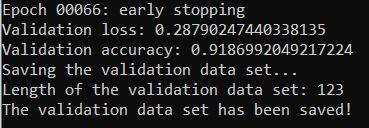
# Get the loss value and metrics values on the validation data set
score = model.evaluate(x_valid, y_valid, verbose=0)
print('Validation loss:', score[0])
print('Validation accuracy:', score[1])
print('Saving the validation data set...')
print('Length of the validation data set:', len(x_valid))
# Go through the validation data set, and see how the model did on each image
for idx in range(len(x_valid)):
# Make the image a NumPy array
img_as_ar = np.array([x_valid[idx]])
# Generate predictions
prediction = model.predict(img_as_ar)
# Determine what the label is based on the highest probability
label = np.argmax(prediction)
# Create the name of the directory and the file for the validation data set
# After each run, delete this out_valid/ directory so that old files are not
# hanging around in there.
file_name = str(idx) + "_" + str(label) + "_" + str(np.argmax(str(y_valid[idx]))) + ".jpg"
img = img_as_ar[0]
# Reverse the image preprocessing process
img = object_detection.reverse_preprocess_inception(img)
# Save the image file
cv2.imwrite(file_name, cv2.cvtColor(img, cv2.COLOR_RGB2BGR))
print('The validation data set has been saved!')
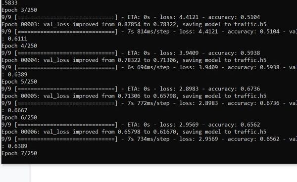
To run the program, type:
python train_traffic_light_color.py
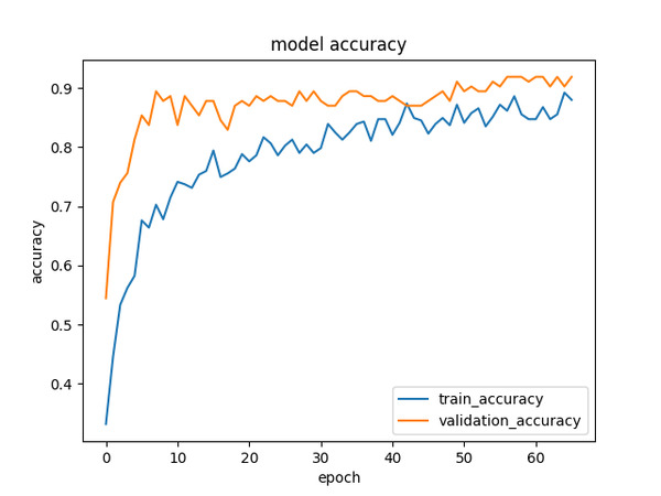
Here is a chart of the accuracy statistics:
Within the current directory, you will now see some new images. These images show how your neural network performed on the validation data set. The second number in the file name indicates the light’s color. Remember:
0 = green
1 = yellow
2 = red
3 = not
My neural network had >92% accuracy in detecting the colors of traffic lights. Pretty good stuff!
In a real self-driving car scenario, we would want to make sure that a traffic light is detected for several frames before labeling it as one color or another.
Note how the training accuracy is worse than the validation accuracy. The reason for this is that we are using image augmentation to artificially expand the data set.
Image augmentation is used during training to help improve the model, but it is also making it harder for the network to get the right answers (i.e. correct traffic light colors) during the training phase of the model.
In contrast, the validation data set is what it is. There is no augmentation, so we are getting higher accuracy values.
To clean up the current working directory, I will cut and paste all these validation data set images into a new folder named output_validation_set.
Test Your Traffic Light Color Detection System on Images
Now that we have our trained neural network saved as traffic.h5, let’s test it out on some fresh images.
Create a new folder inside the main working directory called test_images. Inside that folder, place some images that contain traffic lights. We will see how our network performs on images it hasn’t seen before.
Open a new program called detect_traffic_light_color_img.py. This program will use traffic.h5 and the Single Shot MultiBox Detector to detect traffic light images and annotate their color.
Type the following code:
# Project: How to Detect and Classify Traffic Lights
# Author: Addison Sears-Collins
# Date created: January 17, 2021
# Description: This program uses a trained neural network to
# detect the color of a traffic light in images.

import cv2 # Computer vision library
import numpy as np # Scientific computing library
import object_detection # Custom object detection program
from tensorflow import keras # Library for neural networks
from tensorflow.keras.applications.inception_v3 import InceptionV3, preprocess_input
from tensorflow.keras.applications import imagenet_utils
from tensorflow.keras.preprocessing.image import img_to_array
from tensorflow.keras.preprocessing.image import load_img

FILENAME = "test_red.jpg"

# Load the Inception V3 model
model_inception = InceptionV3(weights='imagenet', include_top=True, input_shape=(299,299,3))

# Resize the image
img = cv2.resize(preprocess_input(cv2.imread(FILENAME)), (299, 299))

# Generate predictions
out_inception = model_inception.predict(np.array([img]))

# Decode the predictions
out_inception = imagenet_utils.decode_predictions(out_inception)

print("Prediction for ", FILENAME , ": ", out_inception[0][0][1], out_inception[0][0][2], "%")

# Show model summary data
model_inception.summary()

# Detect traffic light color in a batch of image files
files = object_detection.get_files('test_images/*.jpg')

# Load the SSD neural network that is trained on the COCO data set
model_ssd = object_detection.load_ssd_coco()

# Load the trained neural network
model_traffic_lights_nn = keras.models.load_model("traffic.h5")

# Go through all image files, and detect the traffic light color.
for file in files:
  (img, out, file_name) = object_detection.perform_object_detection(
    model_ssd, file, save_annotated=True, model_traffic_lights=model_traffic_lights_nn)
  print(file, out)
To run the program, type:
python detect_traffic_light_color_img.py
Test Your Traffic Light Color Detection System on Video
Now that we have tested our traffic light color detection system on images, let’s test it out on video. I have a few mp4 files which I will save to my current directory. One of my videos is named ‘las_vegas.mp4’, and I will save the output video as ‘las_vegas_annotated.mp4’.
Here is the code. I named it detect_traffic_light_color_vid.py.
# Project: How to Detect and Classify Traffic Lights
# Author: Addison Sears-Collins
# Date created: February 1, 2021
# Description: This program uses a trained neural network to
# detect the color of a traffic light in video.

import cv2 # Computer vision library
import numpy as np # Scientific computing library
import object_detection # Custom object detection program
from tensorflow import keras # Library for neural networks
from tensorflow.keras.applications.inception_v3 import InceptionV3, preprocess_input
from tensorflow.keras.applications import imagenet_utils
from tensorflow.keras.preprocessing.image import img_to_array
from tensorflow.keras.preprocessing.image import load_img

# Make sure the video file is in the same directory as your code
filename = 'las_vegas.mp4'
file_size = (1920,1080) # Assumes 1920x1080 mp4
scale_ratio = 1 # Option to scale to fraction of original size.

# We want to save the output to a video file
output_filename = 'las_vegas_annotated.mp4'
output_frames_per_second = 20.0

# Load the SSD neural network that is trained on the COCO data set
model_ssd = object_detection.load_ssd_coco()

# Load the trained neural network
model_traffic_lights_nn = keras.models.load_model("traffic.h5")

def main():

  # Load a video
  cap = cv2.VideoCapture(filename)

  # Create a VideoWriter object so we can save the video output
  fourcc = cv2.VideoWriter_fourcc(*'mp4v')
  result = cv2.VideoWriter(output_filename,
                           fourcc,
                           output_frames_per_second,
                           file_size)

  # Process the video
  while cap.isOpened():

    # Capture one frame at a time
    success, frame = cap.read()

    # Do we have a video frame? If true, proceed.
    if success:

      # Resize the frame
      width = int(frame.shape[1] * scale_ratio)
      height = int(frame.shape[0] * scale_ratio)
      frame = cv2.resize(frame, (width, height))

      # Store the original frame
      original_frame = frame.copy()

      output_frame = object_detection.perform_object_detection_video(
        model_ssd, frame, model_traffic_lights=model_traffic_lights_nn)

      # Write the frame to the output video file
      result.write(output_frame)

    # No more video frames left
    else:
      break

  # Stop when the video is finished
  cap.release()

  # Release the video recording
  result.release()

  # Close all windows
  cv2.destroyAllWindows()

main()
To run the program, type:
python detect_traffic_light_color_vid.py
You will see in the video below that it isn’t perfect. It doesn’t catch all the traffic lights.
To improve performance, I recommend playing around with the score threshold on this line in the object_detection.py code.
if color and label_text and accept_box(output["boxes"], idx, 5.0) and score > 50:
The score is on a threshold of 0 to 100. You can make it 40, for example.
Also, if the color on the traffic lights isn’t accurate, consider adding more training examples, and retraining the color detection neural network on these samples. The more data you have, the better.
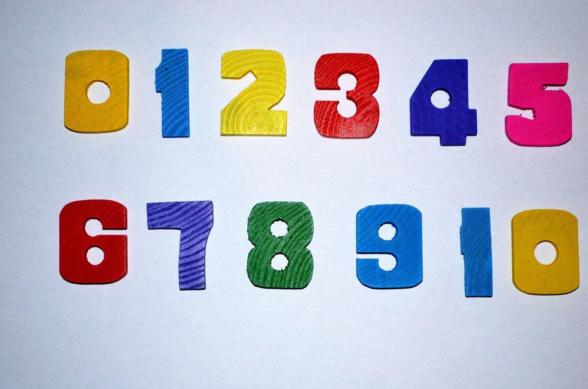
In this tutorial, we will build a convolutional neural network that can classify handwritten digits (i.e. 0 through 9). We will train and test our neural networking using the MNIST data set, a large data set of handwritten digits that is often used as a first project for people who are getting started in deep learning for computer vision.
If you want to use GPU support for your TensorFlow installation, you will need to follow these steps. If you have trouble following those steps, you can follow these steps (note that the steps change quite frequently, but the overall process remains relatively the same).
This post can also help you get your system setup, including your virtual environment in Anaconda (if you decide to go this route).
Directions
Open up a new Python program (in your favorite text editor or Python IDE), and write the following code. I’m going to name the program mnist_handwritten_digits.py.
Here is the code. Don’t be afraid of how long the code is. All you need to do is copy the code and paste it in a file. I included a lot of comments. I’ll explain each piece of the code in detail in a second.
# Project: Detect Handwritten Digits Using the MNIST Data Set
# Author: Addison Sears-Collins
# Date created: January 4, 2021
import tensorflow as tf # Machine learning library
from tensorflow import keras # Library for neural networks
from tensorflow.keras.datasets import mnist # MNIST data set
from tensorflow.keras.layers import Conv2D, Dense, Flatten, MaxPooling2D
from tensorflow.keras.optimizers import Adam
from tensorflow.keras.losses import categorical_crossentropy
import numpy as np
from time import time
import matplotlib.pyplot as plt
num_classes = 10 # Number of distinct labels
def generate_neural_network(x_train):
"""
Create a convolutional neural network.
:x_train: Training images of handwritten digits (grayscale)
:return: Neural network
"""
model = keras.Sequential()
# Add a convolutional layer to the neural network
model.add(Conv2D(filters=6, kernel_size=(
5, 5), activation='relu', padding='same', input_shape=x_train.shape[
1:]))
model.add(MaxPooling2D()) # subsampling using max pooling
# Add a convolutional layer to the neural network
model.add(Conv2D(filters=16, kernel_size=(5, 5), activation='relu'))
model.add(MaxPooling2D())
# Add the dense layers
model.add(Flatten())
model.add(Dense(units=120, activation='relu'))
model.add(Dense(units=84, activation='relu'))
# Softmax transforms the prediction into a probability
# The highest probability corresponds to the category of the image (i.e. 0-9)
model.add(Dense(units=num_classes, activation='softmax'))
return model
def tf_and_gpu_ok():
"""
Test if TensorFlow and GPU support are working properly.
"""
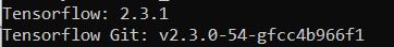
# Test code to see if Tensorflow is installed properly
print("Tensorflow:", tf.__version__)
print("Tensorflow Git:", tf.version.GIT_VERSION)
# See if you can use the GPU on your computer
print("CUDA ON" if tf.test.is_built_with_cuda() else "CUDA OFF")
print("GPU ON" if tf.test.is_gpu_available() else "GPU OFF")
def main():
# Uncomment to check if everything is working properly
#tf_and_gpu_ok()
# Load the MNIST data set and make sure the training and testing
# data are four dimensions (which is what Keras needs)
(x_train, y_train), (x_test, y_test) = mnist.load_data()
x_train = np.reshape(x_train, np.append(x_train.shape, (1)))
x_test = np.reshape(x_test, np.append(x_test.shape, (1)))
# Uncomment to display the dimensions of the training data set and the
# testing data set
#print('x_train', x_train.shape, ' --- x_test', x_test.shape)
#print('y_train', y_train.shape, ' --- y_test', y_test.shape)
# Normalize image intensity values to a range between 0 and 1 (from 0-255)
x_train = x_train.astype('float32')
x_test = x_test.astype('float32')
x_train = x_train / 255
x_test = x_test / 255
# Uncomment to display the first 3 labels
#print('First 3 labels for train set:', y_train[0], y_train[1], y_train[2])
#print('First 3 labels for testing set:', y_test[0], y_test[1], y_test[2])
# Perform one-hot encoding
y_train = keras.utils.to_categorical(y_train, num_classes)
y_test = keras.utils.to_categorical(y_test, num_classes)
# Create the neural network
model = generate_neural_network(x_train)
# Uncomment to print the summary statistics of the neural network
#print(model.summary())
# Configure the neural network
model.compile(loss=categorical_crossentropy, optimizer=Adam(), metrics=['accuracy'])
start = time()
history = model.fit(x_train, y_train, batch_size=16, epochs=5, validation_data=(x_test, y_test), shuffle=True)
training_time = time() - start
print(f'Training time: {training_time}')
# A measure of how well the neural network learned the training data
# The lower, the better
print("Minimum Loss: ", min(history.history['loss']))
# A measure of how well the neural network did on the validation data set
# The lower, the better
print("Minimum Validation Loss: ", min(history.history['val_loss']))
# Maximum percentage of correct predictions on the training data
# The higher, the better
print("Maximum Accuracy: ", max(history.history['accuracy']))
# Maximum percentage of correct predictions on the validation data
# The higher, the better
print("Maximum Validation Accuracy: ", max(history.history['val_accuracy']))
# Plot the key statistics
plt.plot(history.history['loss'])
plt.plot(history.history['val_loss'])
plt.plot(history.history['accuracy'])
plt.plot(history.history['val_accuracy'])
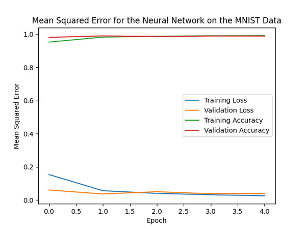
plt.title("Mean Squared Error for the Neural Network on the MNIST Data")
plt.ylabel("Mean Squared Error")
plt.xlabel("Epoch")
plt.legend(['Training Loss', 'Validation Loss', 'Training Accuracy',
'Validation Accuracy'], loc='center right')
plt.show() # Press Q to close the graph
# Save the neural network in Hierarchical Data Format version 5 (HDF5) format
model.save('mnist_nnet.h5')
# Import the saved model
model = keras.models.load_model('mnist_nnet.h5')
print("\n\nNeural network has loaded successfully...\n")
main()
Code Walkthrough
The tf_and_gpu_ok() method is used to check if:
TensorFlow is installed properly.
TensorFlow is able to use the GPU (Graphic Processing Unit) on your computer. The GPU on your computer will help speed up the training of your neural network.
If you see the output below when you run the mnist_handwritten_digits.py program…
python mnist_handwritten_digits.py
…the software is installed correctly.
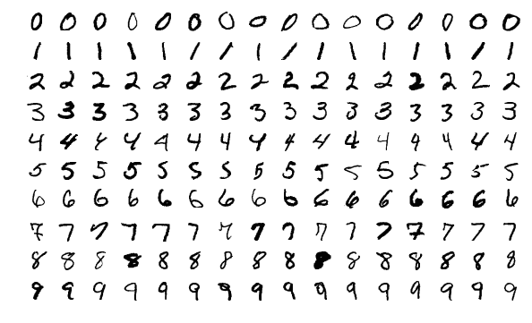
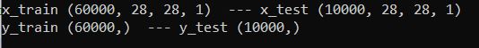
The next piece of code in main displays the dimensions of x_train and y_train. You can see from the output that we train the neural network on 60,000 grayscale images that are 28×28 pixels in size and test the data set on 10,000 grayscale images that are 28×28 pixels in size. Each image contains a handwritten number from 0-9.
At this stage, the intensity for all of the images in the sample ranges from 0-255 (i.e. grayscale). To improve the performance of the neural network, it is helpful to normalize the image intensities to values between 0 and 1. To do this, we need to take the intensity values for each image and divide by the largest value (i.e. 255).
At this stage, we have 10 different labels: 0, 1, 2, 3, 4, 5, 6, 7, 8, 9. These labels represent the 10 different categories (i.e. values) that the handwritten digits could possibly be. To enable the neural network to make better predictions, we need to convert this categorical data into a vector format of just 0s and 1s using a technique known as one-hot encoding.
For each of the 10 possible label values, you get a 10-element vector where only one element is hot (i.e. 1), and the rest of the elements are cold (i.e. 0).
For example, here is the one-hot encoding for the label possibilities in this project:
0 -> 1 0 0 0 0 0 0 0 0 0
1 -> 0 1 0 0 0 0 0 0 0 0
2 -> 0 0 1 0 0 0 0 0 0 0
3 -> 0 0 0 1 0 0 0 0 0 0
4 -> 0 0 0 0 1 0 0 0 0 0
5 -> 0 0 0 0 0 1 0 0 0 0
6 -> 0 0 0 0 0 0 1 0 0 0
7 -> 0 0 0 0 0 0 0 1 0 0
8 -> 0 0 0 0 0 0 0 0 1 0
9 -> 0 0 0 0 0 0 0 0 0 1
Now, we need to generate the neural network. I created a method named generate_neural_network to do just that. If there is something you don’t understand in the code, consult the reference for Keras.
If you want to understand how neural networks make predictions, check out this post.
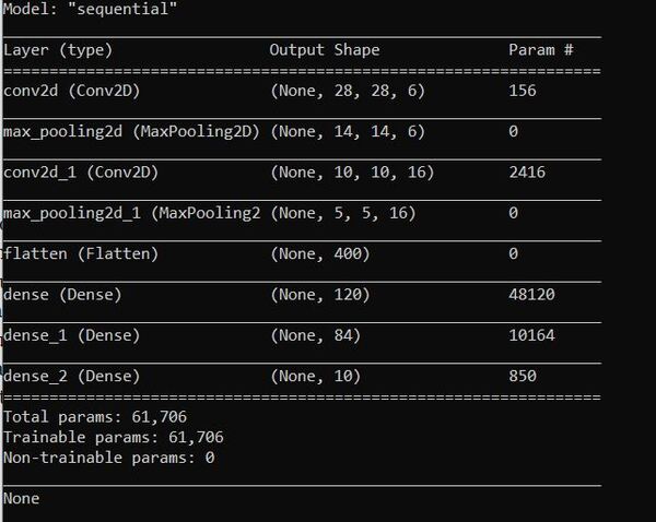
Here is what you will see for the summary statistics:
You can see that the neural network has 61,706 parameters. This number is considerably more than the 4,865 parameters used when we used a deep neural network to predict vehicle fuel economy because we are dealing with images rather than just numbers. As the saying goes, “A picture is worth 1,000 words.”
Now that we have constructed our neural network, we need to train it so that it can be able to make predictions (i.e. convert handwritten numbers into digits 0-9).
We need to feed our network the training samples that consist of the handwritten digits and the corresponding truth (i.e. the labels 0-9). Then we need to train the model and store the data into the history object. If you run the program and hit issues with the version of cuDNN, go to the Anaconda terminal, and type:
conda install -c anaconda cudnn
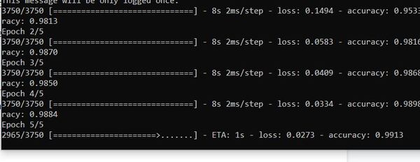
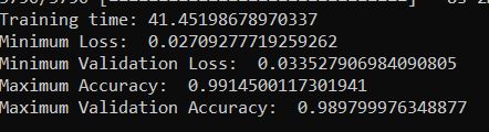
When you run the program, you will see that the accuracy statistics are around 99%.
You should see output on the terminal similar to this graphic when you train the neural network.
At the end of main, I saved our neural network in Hierarchical Data Format version 5 (HDF5) format. I then added some other code to show you how to load the model if you want to do that at a later date.
That’s it! You now know how to build a neural network to accurately classify handwritten digits.


