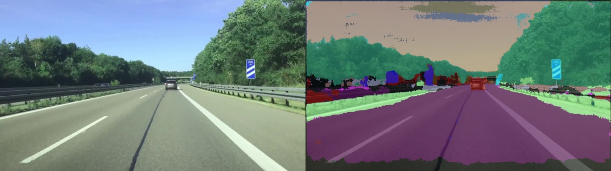
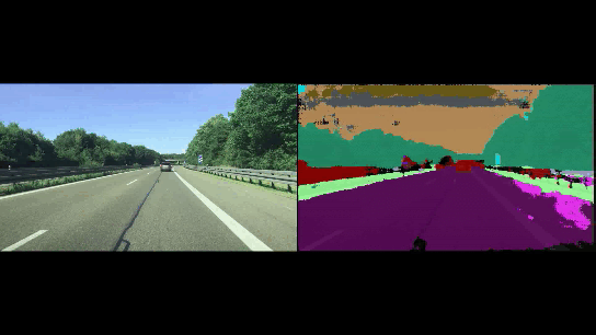
In this tutorial, we will build a program to categorize each pixel in images and videos. These categories could include things like car, person, sidewalk, bicycle, sky, or traffic sign. This process is known as semantic segmentation. By the end of this tutorial, you will be able to generate the following output:

Semantic segmentation helps self-driving cars and other types of autonomous vehicles gain a deep understanding of their surroundings so they can make decisions without human intervention.

Our goal is to build an early prototype of a semantic segmentation application that could be deployed inside an autonomous vehicle. To accomplish this task, we’ll use a special type of neural network called ENet (Efficient Neural Network) (you don’t need to know the details of ENet to accomplish this task).

Here is the list of classes we will use for this project:

Unlabeled
Road
Sidewalk
Building
Wall
Fence
Pole
TrafficLight
TrafficSign
Vegetation
Terrain
Sky
Person
Rider
Car
Truck
Bus
Train
Motorcycle
Bicycle

Real-World Applications

Self-driving cars and other types of autonomous vehicles
Medical (brain and lung tumor detection)

Let’s get started!

Prerequisites

Python 3.7 or higher

Installation and Setup

We now need to make sure we have all the software packages installed. Check to see if you have OpenCV installed on your machine. If you are using Anaconda, you can type:

conda install -c conda-forge opencv

Alternatively, you can type:

pip install opencv-python

Make sure you have NumPy installed, a scientific computing library for Python.

If you’re using Anaconda, you can type:

conda install numpy

Alternatively, you can type:

pip install numpy

Install imutils, an image processing library.

pip install imutils

Download Required Folders and Samples Images and Videos

This link contains the required files you will need to run this program. Download all these files and put them in a folder on your computer.

Code for Semantic Segmentation on Images

In the same folder where you downloaded all the stuff in the previous section, open a new Python file called semantic_segmentation_images.py.

Here is the full code for the system. The only thing you’ll need to change (if you wish to use your own image) in this code is the name of your desired input image file on line 12. Just copy and paste it into your file.

# Project: How To Detect Objects in an Image Using Semantic Segmentation
# Author: Addison Sears-Collins
# Date created: February 24, 2021
# Description: A program that classifies pixels in an image. The real-world
#   use case is autonomous vehicles. Uses the ENet neural network architecture.

import cv2 # Computer vision library
import numpy as np # Scientific computing library 
import os # Operating system library 
import imutils # Image processing library

ORIG_IMG_FILE = 'test_image_1.jpg'
ENET_DIMENSIONS = (1024, 512) # Dimensions that ENet was trained on
RESIZED_WIDTH = 600
IMG_NORM_RATIO = 1 / 255.0 # In grayscale a pixel can range between 0 and 255

# Read the image
input_img = cv2.imread(ORIG_IMG_FILE)

# Resize the image while maintaining the aspect ratio
input_img = imutils.resize(input_img, width=RESIZED_WIDTH)

# Create a blob. A blob is a group of connected pixels in a binary 
# image that share some common property (e.g. grayscale value)
# Preprocess the image to prepare it for deep learning classification
input_img_blob = cv2.dnn.blobFromImage(input_img, IMG_NORM_RATIO,
  ENET_DIMENSIONS, 0, swapRB=True, crop=False)
	
# Load the neural network (i.e. deep learning model)
print("Loading the neural network...")
enet_neural_network = cv2.dnn.readNet('./enet-cityscapes/enet-model.net')

# Set the input for the neural network
enet_neural_network.setInput(input_img_blob)

# Get the predicted probabilities for each of the classes (e.g. car, sidewalk)
# These are the values in the output layer of the neural network
enet_neural_network_output = enet_neural_network.forward()

# Load the names of the classes
class_names = (
  open('./enet-cityscapes/enet-classes.txt').read().strip().split("\n"))

# Print out the shape of the output
# (1, number of classes, height, width)
#print(enet_neural_network_output.shape)

# Extract the key information about the ENet output
(number_of_classes, height, width) = enet_neural_network_output.shape[1:4] 

# number of classes x height x width
#print(enet_neural_network_output[0])

# Find the class label that has the greatest probability for each image pixel
class_map = np.argmax(enet_neural_network_output[0], axis=0)

# Load a list of colors. Each class will have a particular color. 
if os.path.isfile('./enet-cityscapes/enet-colors.txt'):
  IMG_COLOR_LIST = (
    open('./enet-cityscapes/enet-colors.txt').read().strip().split("\n"))
  IMG_COLOR_LIST = [np.array(color.split(",")).astype(
    "int") for color in IMG_COLOR_LIST]
  IMG_COLOR_LIST = np.array(IMG_COLOR_LIST, dtype="uint8")
	
# If the list of colors file does not exist, we generate a 
# random list of colors
else:
  np.random.seed(1)
  IMG_COLOR_LIST = np.random.randint(0, 255, size=(len(class_names) - 1, 3),
    dtype="uint8")
  IMG_COLOR_LIST = np.vstack([[0, 0, 0], IMG_COLOR_LIST]).astype("uint8")
  
# Tie each class ID to its color
# This mask contains the color for each pixel. 
class_map_mask = IMG_COLOR_LIST[class_map]

# We now need to resize the class map mask so its dimensions
# is equivalent to the dimensions of the original image
class_map_mask = cv2.resize(class_map_mask, (
  input_img.shape[1], input_img.shape[0]),
	interpolation=cv2.INTER_NEAREST)

# Overlay the class map mask on top of the original image. We want the mask to
# be transparent. We can do this by computing a weighted average of
# the original image and the class map mask.
enet_neural_network_output = ((0.61 * class_map_mask) + (
  0.39 * input_img)).astype("uint8")
	
# Create a legend that shows the class and its corresponding color
class_legend = np.zeros(((len(class_names) * 25) + 25, 300, 3), dtype="uint8")
	
# Put the class labels and colors on the legend
for (i, (cl_name, cl_color)) in enumerate(zip(class_names, IMG_COLOR_LIST)):
  color_information = [int(color) for color in cl_color]
  cv2.putText(class_legend, cl_name, (5, (i * 25) + 17),
    cv2.FONT_HERSHEY_SIMPLEX, 0.5, (0, 0, 255), 2)
  cv2.rectangle(class_legend, (100, (i * 25)), (300, (i * 25) + 25),
                  tuple(color_information), -1)

# Combine the original image and the semantic segmentation image
combined_images = np.concatenate((input_img, enet_neural_network_output), axis=1) 

# Resize image if desired
#combined_images = imutils.resize(combined_images, width=1000)

# Display image
#cv2.imshow('Results', enet_neural_network_output) 
cv2.imshow('Results', combined_images) 
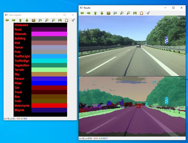
cv2.imshow("Class Legend", class_legend)
print(combined_images.shape)
cv2.waitKey(0) # Display window until keypress
cv2.destroyAllWindows() # Close OpenCV

To run the code, type the following command:

python semantic_segmentation_images.py

Here is the output I got:

How the Code Works

The first thing we need to do is to import the necessary libraries.

import cv2 # Computer vision library
import numpy as np # Scientific computing library 
import os # Operating system library 
import imutils # Image processing library

We set our constants: name of the image file you want to perform semantic segmentation on, the dimensions of the images that the ENet neural network was trained on, the width we want to resize our input image to, and the ratio that we use to normalize the color values of each pixel.

ORIG_IMG_FILE = 'test_image_1.jpg'
ENET_DIMENSIONS = (1024, 512) # Dimensions that ENet was trained on
RESIZED_WIDTH = 600
IMG_NORM_RATIO = 1 / 255.0 # In grayscale a pixel can range between 0 and 255

Read the input image, resize it, and create a blob. A blob is a group of pixels that have similar intensity values.

# Read the image
input_img = cv2.imread(ORIG_IMG_FILE)

# Resize the image while maintaining the aspect ratio
input_img = imutils.resize(input_img, width=RESIZED_WIDTH)

# Create a blob. A blob is a group of connected pixels in a binary 
# image that share some common property (e.g. grayscale value)
# Preprocess the image to prepare it for deep learning classification
input_img_blob = cv2.dnn.blobFromImage(input_img, IMG_NORM_RATIO,
  ENET_DIMENSIONS, 0, swapRB=True, crop=False)

We load the pretrained neural network, set the blob as its input, and then extract the predicted probabilities for each of the classes (i.e. sidewalk, person, car, sky, etc.).

# Load the neural network (i.e. deep learning model)
enet_neural_network = cv2.dnn.readNet('./enet-cityscapes/enet-model.net')

# Set the input for the neural network
enet_neural_network.setInput(input_img_blob)

# Get the predicted probabilities for each of the classes (e.g. car, sidewalk)
# These are the values in the output layer of the neural network
enet_neural_network_output = enet_neural_network.forward()

We load the class list.

# Load the names of the classes
class_names = (
  open('./enet-cityscapes/enet-classes.txt').read().strip().split("\n"))

Get the key parameters of the ENet output.

# Extract the key information about the ENet output
(number_of_classes, height, width) = enet_neural_network_output.shape[1:4]

Determine the highest probability class for each image pixel.

# Find the class label that has the greatest probability for each image pixel
class_map = np.argmax(enet_neural_network_output[0], axis=0)

We want to create a class legend that is color coded.

# Load a list of colors. Each class will have a particular color. 
if os.path.isfile('./enet-cityscapes/enet-colors.txt'):
  IMG_COLOR_LIST = (
    open('./enet-cityscapes/enet-colors.txt').read().strip().split("\n"))
  IMG_COLOR_LIST = [np.array(color.split(",")).astype(
    "int") for color in IMG_COLOR_LIST]
  IMG_COLOR_LIST = np.array(IMG_COLOR_LIST, dtype="uint8")
	
# If the list of colors file does not exist, we generate a 
# random list of colors
else:
  np.random.seed(1)
  IMG_COLOR_LIST = np.random.randint(0, 255, size=(len(class_names) - 1, 3),
    dtype="uint8")
  IMG_COLOR_LIST = np.vstack([[0, 0, 0], IMG_COLOR_LIST]).astype("uint8")

Each pixel will need to have a color, which depends on the highest probability class for that pixel.

# Tie each class ID to its color
# This mask contains the color for each pixel. 
class_map_mask = IMG_COLOR_LIST[class_map]

Make sure the class map mask has the same dimensions as the original input image.

# We now need to resize the class map mask so its dimensions
# is equivalent to the dimensions of the original image
class_map_mask = cv2.resize(class_map_mask, (
  input_img.shape[1], input_img.shape[0]),
	interpolation=cv2.INTER_NEAREST)

Create a blended image of the original input image and the class map mask. In this example, I used 61% of the class map mask and 39% of the original input image. You can change those values, but make sure they add up to 100%.

# Overlay the class map mask on top of the original image. We want the mask to
# be transparent. We can do this by computing a weighted average of
# the original image and the class map mask.
enet_neural_network_output = ((0.61 * class_map_mask) + (
  0.39 * input_img)).astype("uint8")

Create a legend that shows each class and its corresponding color.

# Create a legend that shows the class and its corresponding color
class_legend = np.zeros(((len(class_names) * 25) + 25, 300, 3), dtype="uint8")
	
# Put the class labels and colors on the legend
for (i, (cl_name, cl_color)) in enumerate(zip(class_names, IMG_COLOR_LIST)):
  color_information = [int(color) for color in cl_color]
  cv2.putText(class_legend, cl_name, (5, (i * 25) + 17),
    cv2.FONT_HERSHEY_SIMPLEX, 0.5, (0, 0, 255), 2)
  cv2.rectangle(class_legend, (100, (i * 25)), (300, (i * 25) + 25),
                  tuple(color_information), -1)

Create the final image we want to display. The original input image is combined with the semantic segmentation image.

# Combine the original image and the semantic segmentation image
combined_images = np.concatenate((input_img, enet_neural_network_output), axis=0)

Display the image.

# Display image
#cv2.imshow('Results', enet_neural_network_output) 
cv2.imshow('Results', combined_images) 
cv2.imshow("Class Legend", class_legend)
print(combined_images.shape)
cv2.waitKey(0) # Display window until keypress
cv2.destroyAllWindows() # Close OpenCV

Code for Semantic Segmentation on Videos

Open a new Python file called semantic_segmentation_videos.py.

Here is the full code for the system. The only thing you’ll need to change (if you wish to use your own video) in this code is the name of your desired input video file on line 13, and the name of your desired output video file on line 17. Make sure the input video is 1920 x 1080 pixels in dimensions and is in mp4 format, otherwise it won’t work.

# Project: How To Detect Objects in a Video Using Semantic Segmentation
# Author: Addison Sears-Collins
# Date created: February 25, 2021
# Description: A program that classifies pixels in a video. The real-world
#   use case is autonomous vehicles. Uses the ENet neural network architecture.

import cv2 # Computer vision library
import numpy as np # Scientific computing library 
import os # Operating system library 
import imutils # Image processing library

# Make sure the video file is in the same directory as your code
filename = '4_orig_lane_detection_1.mp4'
file_size = (1920,1080) # Assumes 1920x1080 mp4

# We want to save the output to a video file
output_filename = 'semantic_seg_4_orig_lane_detection_1.mp4'
output_frames_per_second = 20.0 

ENET_DIMENSIONS = (1024, 512) # Dimensions that ENet was trained on
RESIZED_WIDTH = 1200
IMG_NORM_RATIO = 1 / 255.0 # In grayscale a pixel can range between 0 and 255

# Load the names of the classes
class_names = (
  open('./enet-cityscapes/enet-classes.txt').read().strip().split("\n"))
	
# Load a list of colors. Each class will have a particular color. 
if os.path.isfile('./enet-cityscapes/enet-colors.txt'):
  IMG_COLOR_LIST = (
    open('./enet-cityscapes/enet-colors.txt').read().strip().split("\n"))
  IMG_COLOR_LIST = [np.array(color.split(",")).astype(
    "int") for color in IMG_COLOR_LIST]
  IMG_COLOR_LIST = np.array(IMG_COLOR_LIST, dtype="uint8")
	
# If the list of colors file does not exist, we generate a 
# random list of colors
else:
  np.random.seed(1)
  IMG_COLOR_LIST = np.random.randint(0, 255, size=(len(class_names) - 1, 3),
    dtype="uint8")
  IMG_COLOR_LIST = np.vstack([[0, 0, 0], IMG_COLOR_LIST]).astype("uint8")

def main():

  # Load a video
  cap = cv2.VideoCapture(filename)

  # Create a VideoWriter object so we can save the video output
  fourcc = cv2.VideoWriter_fourcc(*'mp4v')
  result = cv2.VideoWriter(output_filename,  
                           fourcc, 
                           output_frames_per_second, 
                           file_size) 
	
  # Process the video
  while cap.isOpened():
		
    # Capture one frame at a time
    success, frame = cap.read() 
		
    # Do we have a video frame? If true, proceed.
    if success:
		
      # Resize the frame while maintaining the aspect ratio
      frame = imutils.resize(frame, width=RESIZED_WIDTH)

      # Create a blob. A blob is a group of connected pixels in a binary 
      # frame that share some common property (e.g. grayscale value)
      # Preprocess the frame to prepare it for deep learning classification
      frame_blob = cv2.dnn.blobFromImage(frame, IMG_NORM_RATIO,
                     ENET_DIMENSIONS, 0, swapRB=True, crop=False)
	
      # Load the neural network (i.e. deep learning model)
      enet_neural_network = cv2.dnn.readNet('./enet-cityscapes/enet-model.net')

      # Set the input for the neural network
      enet_neural_network.setInput(frame_blob)

      # Get the predicted probabilities for each of 
      # the classes (e.g. car, sidewalk)
      # These are the values in the output layer of the neural network
      enet_neural_network_output = enet_neural_network.forward()

      # Extract the key information about the ENet output
      (number_of_classes, height, width) = (
        enet_neural_network_output.shape[1:4]) 

      # Find the class label that has the greatest 
      # probability for each frame pixel
      class_map = np.argmax(enet_neural_network_output[0], axis=0)

      # Tie each class ID to its color
      # This mask contains the color for each pixel. 
      class_map_mask = IMG_COLOR_LIST[class_map]

      # We now need to resize the class map mask so its dimensions
      # is equivalent to the dimensions of the original frame
      class_map_mask = cv2.resize(class_map_mask, (
        frame.shape[1], frame.shape[0]), 
        interpolation=cv2.INTER_NEAREST)

      # Overlay the class map mask on top of the original frame. We want 
      # the mask to be transparent. We can do this by computing a weighted 
      # average of the original frame and the class map mask.
      enet_neural_network_output = ((0.90 * class_map_mask) + (
        0.10 * frame)).astype("uint8")
	
      # Combine the original frame and the semantic segmentation frame
      combined_frames = np.concatenate(
        (frame, enet_neural_network_output), axis=1) 

      # Resize frame if desired
      combined_frames = imutils.resize(combined_frames, width=1920)

      # Create an appropriately-sized video frame. We want the video height
      # to be 1080 pixels
      adjustment_for_height = 1080 - combined_frames.shape[0]
      adjustment_for_height = int(adjustment_for_height / 2)
      black_img_1 = np.zeros((adjustment_for_height, 1920, 3), dtype = "uint8")
      black_img_2 = np.zeros((adjustment_for_height, 1920, 3), dtype = "uint8")

      # Add black padding to the video frame on the top and bottom
      combined_frames = np.concatenate((black_img_1, combined_frames), axis=0) 
      combined_frames = np.concatenate((combined_frames, black_img_2), axis=0) 
      
			# Write the frame to the output video file
      result.write(combined_frames)
		
    # No more video frames left
    else:
      break
			
  # Stop when the video is finished
  cap.release()
	
  # Release the video recording
  result.release()

main()

To run the code, type the following command:

python semantic_segmentation_videos.py

Video Output

Here is the output:

How the Code Works

This code is pretty much the same as the code for images. The only difference is that we run the algorithm on each frame of the input video rather than a single input image.

I put detailed comments inside the code so that you can understand what is going on.

That’s it. Keep building!