In this tutorial, we will learn how to track multiple objects in a video using OpenCV, the computer vision library for Python. By the end of this tutorial, you will be able to generate the following output:
Real-World Applications
Object tracking has a number of real-world use cases. Here are a few:
- Drone Surveillance
- Aerial Cinematography
- Tracking Customers to Understand In-Store Consumer Behavior
- Any Kind of Robot That You Want to Follow You as You Move Around
Let’s get started!
Prerequisites
Installation and Setup
We first need to make sure we have all the software packages installed. Check to see if you have OpenCV installed on your machine. If you are using Anaconda, you can type:
conda install -c conda-forge opencv
Alternatively, you can type:
pip install opencv-python
Find Video Files
Find a video file that contains objects you would like to detect. I suggest finding a file that is 1920 x 1080 pixels in dimensions and is in mp4 format. You can find some good videos at sites like Pixabay.com and Pexels.com.
Save the video file in a folder somewhere on your computer.
Write the Code
Navigate to the directory where you saved your video, and open a new Python program named multi_object_tracking.py.
Here is the full code for the program. You can copy and paste this code directly into your program. The only line you will need to change is line 10. The video file I’m using is named fish.mp4, so I will write ‘fish’ as the file prefix.
If your video is not 1920 x 1080 dimensions, you will need to modify line 12 accordingly.
# Project: How to Do Multiple Object Tracking Using OpenCV
# Author: Addison Sears-Collins
# Date created: March 2, 2021
# Description: Tracking multiple objects in a video using OpenCV
import cv2 # Computer vision library
from random import randint # Handles the creation of random integers
# Make sure the video file is in the same directory as your code
file_prefix = 'fish'
filename = file_prefix + '.mp4'
file_size = (1920,1080) # Assumes 1920x1080 mp4
# We want to save the output to a video file
output_filename = file_prefix + '_object_tracking.mp4'
output_frames_per_second = 20.0
# OpenCV has a bunch of object tracking algorithms. We list them here.
type_of_trackers = ['BOOSTING', 'MIL', 'KCF','TLD', 'MEDIANFLOW', 'GOTURN',
'MOSSE', 'CSRT']
# CSRT is accurate but slow. You can try others and see what results you get.
desired_tracker = 'CSRT'
# Generate a MultiTracker object
multi_tracker = cv2.MultiTracker_create()
# Set bounding box drawing parameters
from_center = False # Draw bounding box from upper left
show_cross_hair = False # Don't show the cross hair
def generate_tracker(type_of_tracker):
"""
Create object tracker.
:param type_of_tracker string: OpenCV tracking algorithm
"""
if type_of_tracker == type_of_trackers[0]:
tracker = cv2.TrackerBoosting_create()
elif type_of_tracker == type_of_trackers[1]:
tracker = cv2.TrackerMIL_create()
elif type_of_tracker == type_of_trackers[2]:
tracker = cv2.TrackerKCF_create()
elif type_of_tracker == type_of_trackers[3]:
tracker = cv2.TrackerTLD_create()
elif type_of_tracker == type_of_trackers[4]:
tracker = cv2.TrackerMedianFlow_create()
elif type_of_tracker == type_of_trackers[5]:
tracker = cv2.TrackerGOTURN_create()
elif type_of_tracker == type_of_trackers[6]:
tracker = cv2.TrackerMOSSE_create()
elif type_of_tracker == type_of_trackers[7]:
tracker = cv2.TrackerCSRT_create()
else:
tracker = None
print('The name of the tracker is incorrect')
print('Here are the possible trackers:')
for track_type in type_of_trackers:
print(track_type)
return tracker
def main():
# Load a video
cap = cv2.VideoCapture(filename)
# Create a VideoWriter object so we can save the video output
fourcc = cv2.VideoWriter_fourcc(*'mp4v')
result = cv2.VideoWriter(output_filename,
fourcc,
output_frames_per_second,
file_size)
# Capture the first video frame
success, frame = cap.read()
bounding_box_list = []
color_list = []
# Do we have a video frame? If true, proceed.
if success:
while True:
# Draw a bounding box over all the objects that you want to track_type
# Press ENTER or SPACE after you've drawn the bounding box
bounding_box = cv2.selectROI('Multi-Object Tracker', frame, from_center,
show_cross_hair)
# Add a bounding box
bounding_box_list.append(bounding_box)
# Add a random color_list
blue = 255 # randint(127, 255)
green = 0 # randint(127, 255)
red = 255 #randint(127, 255)
color_list.append((blue, green, red))
# Press 'q' (make sure you click on the video frame so that it is the
# active window) to start object tracking. You can press another key
# if you want to draw another bounding box.
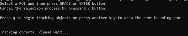
print("\nPress q to begin tracking objects or press " +
"another key to draw the next bounding box\n")
# Wait for keypress
k = cv2.waitKey() & 0xFF
# Start tracking objects if 'q' is pressed
if k == ord('q'):
break
cv2.destroyAllWindows()
print("\nTracking objects. Please wait...")
# Set the tracker
type_of_tracker = desired_tracker
for bbox in bounding_box_list:
# Add tracker to the multi-object tracker
multi_tracker.add(generate_tracker(type_of_tracker), frame, bbox)
# Process the video
while cap.isOpened():
# Capture one frame at a time
success, frame = cap.read()
# Do we have a video frame? If true, proceed.
if success:
# Update the location of the bounding boxes
success, bboxes = multi_tracker.update(frame)
# Draw the bounding boxes on the video frame
for i, bbox in enumerate(bboxes):
point_1 = (int(bbox[0]), int(bbox[1]))
point_2 = (int(bbox[0] + bbox[2]),
int(bbox[1] + bbox[3]))
cv2.rectangle(frame, point_1, point_2, color_list[i], 5)
# Write the frame to the output video file
result.write(frame)
# No more video frames left
else:
break
# Stop when the video is finished
cap.release()
# Release the video recording
result.release()
main()
Run the Code
Launch the program.
python multi_object_tracking.py
The first frame of the video will pop up. With this frame selected, grab your mouse, and draw a rectangle around the object you would like to track.
When you’re done drawing the rectangle, press Enter or Space.
If you just want to track this object, press ‘q’ to run the program’. Otherwise, if you want to track more objects, press any other key to draw some more rectangles around other objects you want to track.
After you press ‘q’, the program will run. Once the program is finished doing its job, you will have a new video file. It will be named something like fish_object_tracking.mp4. This file is your final video output.
Video Output
Here is my final video:
How the Code Works
OpenCV has a number of object trackers: ‘BOOSTING’, ‘MIL’, ‘KCF’,’TLD’, ‘MEDIANFLOW’, ‘GOTURN’, ‘MOSSE’, ‘CSRT’. In our implementation, we used CSRT which is slow but accurate.
When we run the program, the first video frame is captured. We have to identify the object(s) we want to track by drawing a rectangle around it. After we do that, the algorithm tracks the object through each frame of the video.
Once the program has finished processing all video frames, the annotated video is saved to your computer.
That’s it. Keep building!