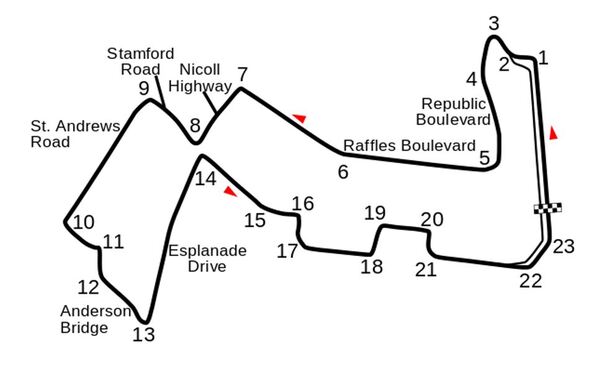
I recently built a project to combine the Extended Kalman Filter (for state estimation) and the Linear Quadratic Regulator (for control) to drive a simulated path-following race car (which is modeled as a point) around a track that is the same shape as the Formula 1 Singapore Grand Prix Marina Bay Street Circuit race track.
How the Program Works
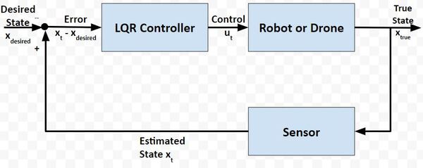
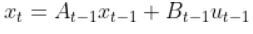
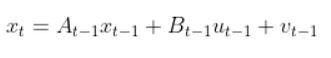
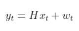
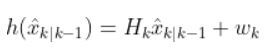
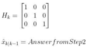
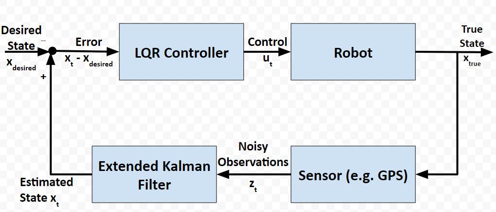
In a real-world application, it is common for a robot to use the Extended Kalman Filter to calculate near-optimal estimates of the state of a robotic system and to use LQR to generate the control values that move the robot from one state to the next.
Here is a block diagram of that process:
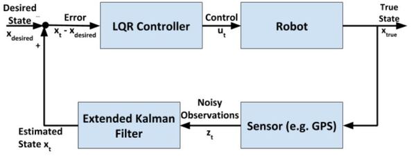
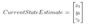
At each timestep:
- Control commands are sent by the LQR algorithm
- The robot changes state
- Sensor measurements are made
- The sensor measurements are used to generate near-optimal estimates of the state
- These estimates of the state get fed into the LQR controller to determine what the next control commands should be
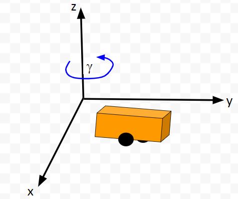
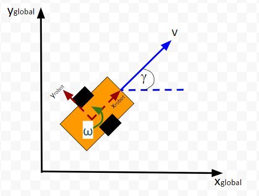
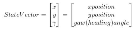
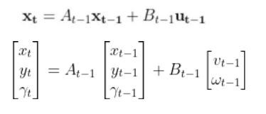
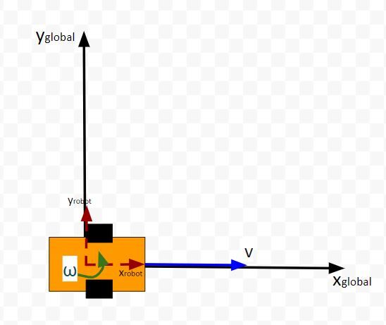
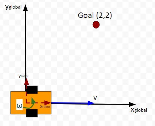
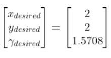
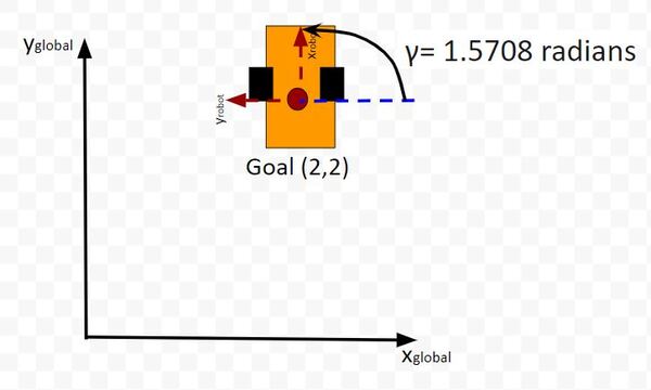
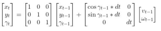
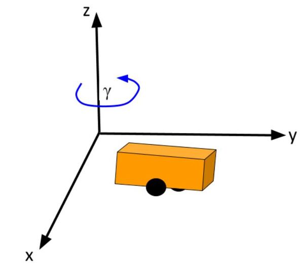
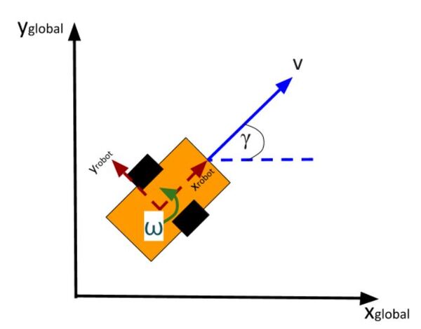
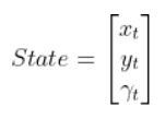
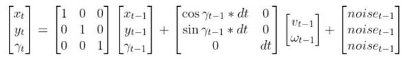
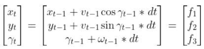
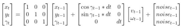
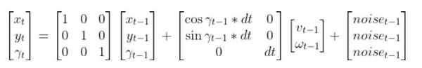
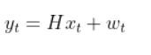
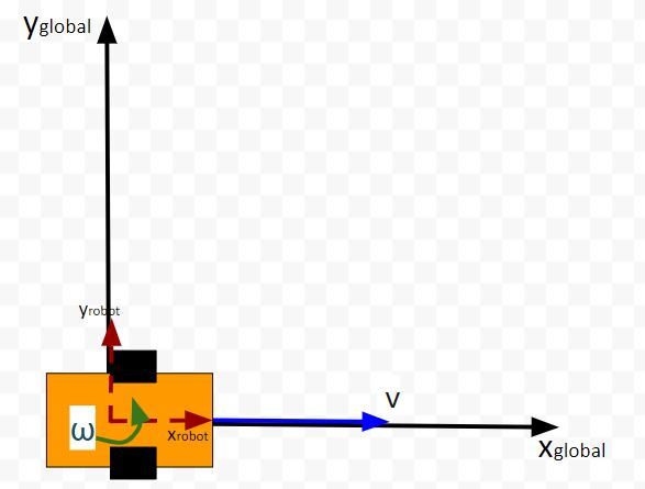
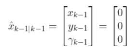
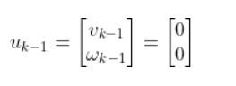
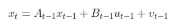
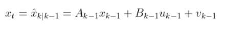
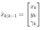
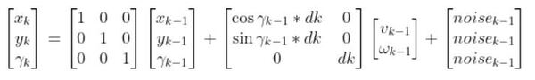
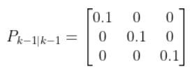
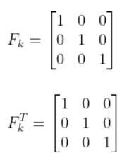
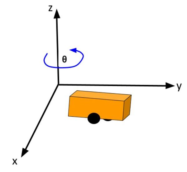
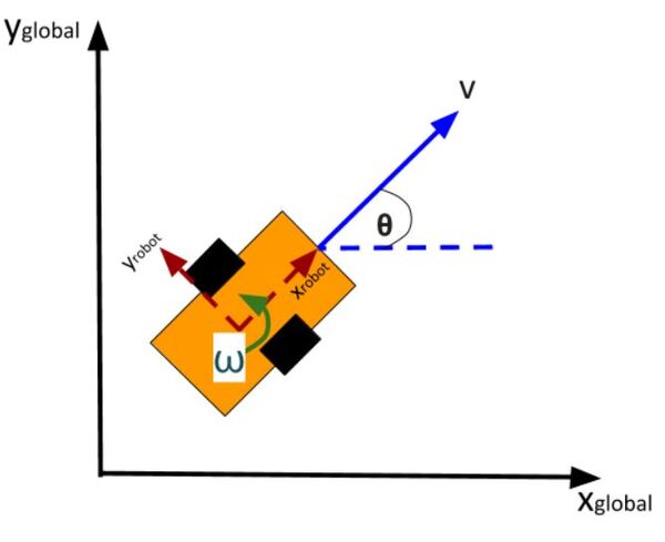
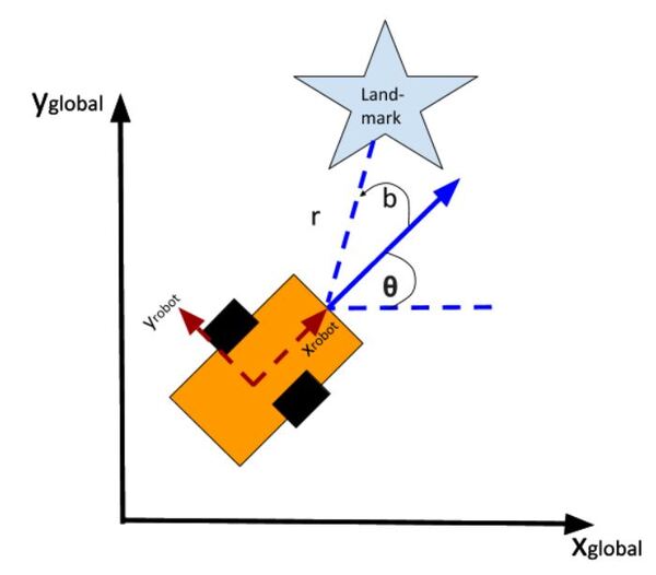
The kinematics of the system are modeled according to the following diagrams:
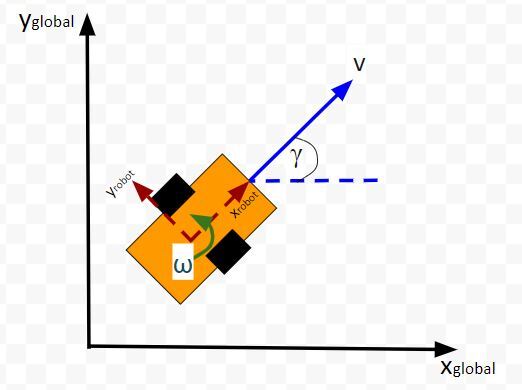
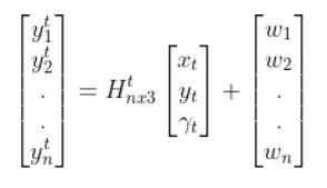
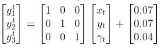
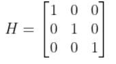
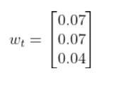
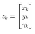
In my application, I assume there are sensors mounted on the race car that help it to localize itself in the x-y coordinate plane. These sensors measure the range (r) and bearing (b) from the race car to each landmark. Each landmark has a known x and y position.
The programs I developed were written in Python and use the same sequence of actions as indicated in the block diagram (in the first part of this post) in order to follow the race track (which is a list of waypoints).
Code
You will need to put these five Python (3.7 or higher) programs into a single directory.
cubic_spine_planner.py
"""
Cubic spline planner

Program: cubic_spine_planner.py

Author: Atsushi Sakai(@Atsushi_twi)
Source: https://github.com/AtsushiSakai/PythonRobotics

This program implements a cubic spline. For more information on
cubic splines, check out this link:
https://mathworld.wolfram.com/CubicSpline.html
"""
import math
import numpy as np
import bisect

class Spline:
    """
    Cubic Spline class
    """

    def __init__(self, x, y):
        self.b, self.c, self.d, self.w = [], [], [], []

        self.x = x
        self.y = y

        self.nx = len(x)  # dimension of x
        h = np.diff(x)

        # calc coefficient c
        self.a = [iy for iy in y]

        # calc coefficient c
        A = self.__calc_A(h)
        B = self.__calc_B(h)
        self.c = np.linalg.solve(A, B)
        #  print(self.c1)

        # calc spline coefficient b and d
        for i in range(self.nx - 1):
            self.d.append((self.c[i + 1] - self.c[i]) / (3.0 * h[i]))
            tb = (self.a[i + 1] - self.a[i]) / h[i] - h[i] * \
                (self.c[i + 1] + 2.0 * self.c[i]) / 3.0
            self.b.append(tb)

    def calc(self, t):
        """
        Calc position

        if t is outside of the input x, return None

        """

        if t < self.x[0]:
            return None
        elif t > self.x[-1]:
            return None

        i = self.__search_index(t)
        dx = t - self.x[i]
        result = self.a[i] + self.b[i] * dx + \
            self.c[i] * dx ** 2.0 + self.d[i] * dx ** 3.0

        return result

    def calcd(self, t):
        """
        Calc first derivative

        if t is outside of the input x, return None
        """

        if t < self.x[0]:
            return None
        elif t > self.x[-1]:
            return None

        i = self.__search_index(t)
        dx = t - self.x[i]
        result = self.b[i] + 2.0 * self.c[i] * dx + 3.0 * self.d[i] * dx ** 2.0
        return result

    def calcdd(self, t):
        """
        Calc second derivative
        """

        if t < self.x[0]:
            return None
        elif t > self.x[-1]:
            return None

        i = self.__search_index(t)
        dx = t - self.x[i]
        result = 2.0 * self.c[i] + 6.0 * self.d[i] * dx
        return result

    def __search_index(self, x):
        """
        search data segment index
        """
        return bisect.bisect(self.x, x) - 1

    def __calc_A(self, h):
        """
        calc matrix A for spline coefficient c
        """
        A = np.zeros((self.nx, self.nx))
        A[0, 0] = 1.0
        for i in range(self.nx - 1):
            if i != (self.nx - 2):
                A[i + 1, i + 1] = 2.0 * (h[i] + h[i + 1])
            A[i + 1, i] = h[i]
            A[i, i + 1] = h[i]

        A[0, 1] = 0.0
        A[self.nx - 1, self.nx - 2] = 0.0
        A[self.nx - 1, self.nx - 1] = 1.0
        #  print(A)
        return A

    def __calc_B(self, h):
        """
        calc matrix B for spline coefficient c
        """
        B = np.zeros(self.nx)
        for i in range(self.nx - 2):
            B[i + 1] = 3.0 * (self.a[i + 2] - self.a[i + 1]) / \
                h[i + 1] - 3.0 * (self.a[i + 1] - self.a[i]) / h[i]
        return B


class Spline2D:
    """
    2D Cubic Spline class

    """

    def __init__(self, x, y):
        self.s = self.__calc_s(x, y)
        self.sx = Spline(self.s, x)
        self.sy = Spline(self.s, y)

    def __calc_s(self, x, y):
        dx = np.diff(x)
        dy = np.diff(y)
        self.ds = [math.sqrt(idx ** 2 + idy ** 2)
                   for (idx, idy) in zip(dx, dy)]
        s = [0]
        s.extend(np.cumsum(self.ds))
        return s

    def calc_position(self, s):
        """
        calc position
        """
        x = self.sx.calc(s)
        y = self.sy.calc(s)

        return x, y

    def calc_curvature(self, s):
        """
        calc curvature
        """
        dx = self.sx.calcd(s)
        ddx = self.sx.calcdd(s)
        dy = self.sy.calcd(s)
        ddy = self.sy.calcdd(s)
        k = (ddy * dx - ddx * dy) / ((dx ** 2 + dy ** 2)**(3 / 2))
        return k

    def calc_yaw(self, s):
        """
        calc yaw
        """
        dx = self.sx.calcd(s)
        dy = self.sy.calcd(s)
        yaw = math.atan2(dy, dx)
        return yaw


def calc_spline_course(x, y, ds=0.1):
    sp = Spline2D(x, y)
    s = list(np.arange(0, sp.s[-1], ds))

    rx, ry, ryaw, rk = [], [], [], []
    for i_s in s:
        ix, iy = sp.calc_position(i_s)
        rx.append(ix)
        ry.append(iy)
        ryaw.append(sp.calc_yaw(i_s))
        rk.append(sp.calc_curvature(i_s))

    return rx, ry, ryaw, rk, s


def main():
    print("Spline 2D test")
    import matplotlib.pyplot as plt
    x = [-2.5, 0.0, 2.5, 5.0, 7.5, 3.0, -1.0]
    y = [0.7, -6, 5, 6.5, 0.0, 5.0, -2.0]
    ds = 0.1  # [m] distance of each intepolated points

    sp = Spline2D(x, y)
    s = np.arange(0, sp.s[-1], ds)

    rx, ry, ryaw, rk = [], [], [], []
    for i_s in s:
        ix, iy = sp.calc_position(i_s)
        rx.append(ix)
        ry.append(iy)
        ryaw.append(sp.calc_yaw(i_s))
        rk.append(sp.calc_curvature(i_s))

    flg, ax = plt.subplots(1)
    plt.plot(x, y, "xb", label="input")
    plt.plot(rx, ry, "-r", label="spline")
    plt.grid(True)
    plt.axis("equal")
    plt.xlabel("x[m]")
    plt.ylabel("y[m]")
    plt.legend()

    flg, ax = plt.subplots(1)
    plt.plot(s, [math.degrees(iyaw) for iyaw in ryaw], "-r", label="yaw")
    plt.grid(True)
    plt.legend()
    plt.xlabel("line length[m]")
    plt.ylabel("yaw angle[deg]")

    flg, ax = plt.subplots(1)
    plt.plot(s, rk, "-r", label="curvature")
    plt.grid(True)
    plt.legend()
    plt.xlabel("line length[m]")
    plt.ylabel("curvature [1/m]")

    plt.show()

if __name__ == '__main__':
    main()
kinematics.py
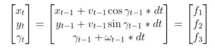
"""
Implementation of the two-wheeled differential drive robot car
and its controller.
Our goal in using LQR is to find the optimal control inputs:
[linear velocity of the car, angular velocity of the car]
We want to both minimize the error between the current state
and a desired state, while minimizing actuator effort
(e.g. wheel rotation rate). These are competing objectives because a
large u (i.e. wheel rotation rates) expends a lot of
actuator energy but can drive the state error to 0 really fast.
LQR helps us balance these competing objectives.
If a system is linear, LQR gives the optimal control inputs that
takes a system's state to 0, where the state is
"current state - desired state".
Implemented by Addison Sears-Collins
Date: December 10, 2020
"""
# Import required libraries
import numpy as np
import scipy.linalg as la
class DifferentialDrive(object):
"""
Implementation of Differential Drive kinematics.
This represents a two-wheeled vehicle defined by the following states
state = [x,y,theta] where theta is the yaw angle
and accepts the following control inputs
input = [linear velocity of the car, angular velocity of the car]
"""
def __init__(self):
"""
Initializes the class
"""
# Covariance matrix representing action noise
# (i.e. noise on the control inputs)
self.V = None
def get_state_size(self):
"""
The state is (X, Y, THETA) in global coordinates, so the state size is 3.
"""
return 3
def get_input_size(self):
"""
The control input is ([linear velocity of the car, angular velocity of the car]),
so the input size is 2.
"""
return 2
def get_V(self):
"""
This function provides the covariance matrix V which
describes the noise that can be applied to the forward kinematics.
Feel free to experiment with different levels of noise.
Output
:return: V: input cost matrix (3 x 3 matrix)
"""
# The np.eye function returns a 2D array with ones on the diagonal
# and zeros elsewhere.
if self.V is None:
self.V = np.eye(3)
self.V[0,0] = 0.01
self.V[1,1] = 0.01
self.V[2,2] = 0.1
return 1e-5*self.V
def forward(self,x0,u,v,dt=0.1):
"""
Computes the forward kinematics for the system.
Input
:param x0: The starting state (position) of the system (units:[m,m,rad])
np.array with shape (3,) ->
(X, Y, THETA)
:param u: The control input to the system
2x1 NumPy Array given the control input vector is
[linear velocity of the car, angular velocity of the car]
[meters per second, radians per second]
:param v: The noise applied to the system (units:[m, m, rad]) ->np.array
with shape (3,)
:param dt: Change in time (units: [s])
Output
:return: x1: The new state of the system (X, Y, THETA)
"""
u0 = u
# If there is no noise applied to the system
if v is None:
v = 0
# Starting state of the vehicle
X = x0[0]
Y = x0[1]
THETA = x0[2]
# Control input
u_linvel = u0[0]
u_angvel = u0[1]
# Velocity in the x and y direction in m/s
x_dot = u_linvel * np.cos(THETA)
y_dot = u_linvel * np.sin(THETA)
# The new state of the system
x1 = np.empty(3)
# Calculate the new state of the system
# Noise is added like in slide 34 in Lecture 7
x1[0] = x0[0] + x_dot * dt + v[0] # X
x1[1] = x0[1] + y_dot * dt + v[1] # Y
x1[2] = x0[2] + u_angvel * dt + v[2] # THETA
return x1
def linearize(self, x, dt=0.1):
"""
Creates a linearized version of the dynamics of the differential
drive robotic system (i.e. a
robotic car where each wheel is controlled separately.
The system's forward kinematics are nonlinear due to the sines and
cosines, so we need to linearize
it by taking the Jacobian of the forward kinematics equations with respect
to the control inputs.
Our goal is to have a discrete time system of the following form:
x_t+1 = Ax_t + Bu_t where:
Input
:param x: The state of the system (units:[m,m,rad]) ->
np.array with shape (3,) ->
(X, Y, THETA) ->
X_system = [x1, x2, x3]
:param dt: The change in time from time step t to time step t+1
Output
:return: A: Matrix A is a 3x3 matrix (because there are 3 states) that
describes how the state of the system changes from t to t+1
when no control command is executed. Typically,
a robotic car only drives when the wheels are turning.
Therefore, in this case, A is the identity matrix.
:return: B: Matrix B is a 3 x 2 matrix (because there are 3 states and
2 control inputs) that describes how
the state (X, Y, and THETA) changes from t to t + 1 due to
the control command u.
Matrix B is found by taking the The Jacobian of the three
forward kinematics equations (for X, Y, THETA)
with respect to u (3 x 2 matrix)
"""
THETA = x[2]
####### A Matrix #######
# A matrix is the identity matrix
A = np.array([[1.0, 0, 0],
[ 0, 1.0, 0],
[ 0, 0, 1.0]])
####### B Matrix #######
B = np.array([[np.cos(THETA)*dt, 0],
[np.sin(THETA)*dt, 0],
[0, dt]])
return A, B
def dLQR(F,Q,R,x,xf,dt=0.1):
"""
Discrete-time linear quadratic regulator for a non-linear system.
Compute the optimal control given a nonlinear system, cost matrices,
a current state, and a final state.
Compute the control variables that minimize the cumulative cost.
Solve for P using the dynamic programming method.
Assume that Qf = Q
Input:
:param F: The dynamics class object (has forward and linearize functions
implemented)
:param Q: The state cost matrix Q -> np.array with shape (3,3)
:param R: The input cost matrix R -> np.array with shape (2,2)
:param x: The current state of the system x -> np.array with shape (3,)
:param xf: The desired state of the system xf -> np.array with shape (3,)
:param dt: The size of the timestep -> float
Output
:return: u_t_star: Optimal action u for the current state
[linear velocity of the car, angular velocity of the car]
[meters per second, radians per second]
"""
# We want the system to stabilize at xf,
# so we let x - xf be the state.
# Actual state - desired state
x_error = x - xf
# Calculate the A and B matrices
A, B = F.linearize(x, dt)
# Solutions to discrete LQR problems are obtained using dynamic
# programming.
# The optimal solution is obtained recursively, starting at the last
# time step and working backwards.
N = 50
# Create a list of N + 1 elements
P = [None] * (N + 1)
# Assume Qf = Q
Qf = Q
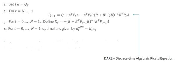
# 1. LQR via Dynamic Programming
P[N] = Qf
# 2. For t = N, ..., 1
for t in range(N, 0, -1):
# Discrete-time Algebraic Riccati equation to calculate the optimal
# state cost matrix
P[t-1] = Q + A.T @ P[t] @ A - (A.T @ P[t] @ B) @ la.pinv(
R + B.T @ P[t] @ B) @ (B.T @ P[t] @ A)
# Create a list of N elements
K = [None] * N
u = [None] * N
# 3 and 4. For t = 0, ..., N - 1
for t in range(N):
# Calculate the optimal feedback gain K_t
K[t] = -la.pinv(R + B.T @ P[t+1] @ B) @ B.T @ P[t+1] @ A
for t in range(N):
# Calculate the optimal control input
u[t] = K[t] @ x_error
# Optimal control input is u_t_star
u_t_star = u[N-1]
# Return the optimal control inputs
return u_t_star
def get_R():
"""
This function provides the R matrix to the lqr_ekf_control simulator.
Returns the input cost matrix R.
Experiment with different gains.
This matrix penalizes actuator effort
(i.e. rotation of the motors on the wheels).
The R matrix has the same number of rows as are actuator states
[linear velocity of the car, angular velocity of the car]
[meters per second, radians per second]
This matrix often has positive values along the diagonal.
We can target actuator states where we want low actuator
effort by making the corresponding value of R large.
Output
:return: R: Input cost matrix
"""
R = np.array([[0.01, 0], # Penalization for linear velocity effort
[0, 0.01]]) # Penalization for angular velocity effort
return R
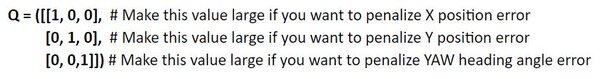
def get_Q():
"""
This function provides the Q matrix to the lqr_ekf_control simulator.
Returns the state cost matrix Q.
Experiment with different gains to see their effect on the vehicle's
behavior.
Q helps us weight the relative importance of each state in the state
vector (X, Y, THETA).
Q is a square matrix that has the same number of rows as there are states.
Q penalizes bad performance.
Q has positive values along the diagonal and zeros elsewhere.
Q enables us to target states where we want low error by making the
corresponding value of Q large.
We can start with the identity matrix and tweak the values through trial
and error.
Output
:return: Q: State cost matrix (3x3 matrix because the state vector is
(X, Y, THETA))
"""
Q = np.array([[0.4, 0, 0], # Penalize X position error (global coordinates)
[0, 0.4, 0], # Penalize Y position error (global coordinates)
[0, 0, 0.4]])# Penalize heading error (global coordinates)
return Q
lqr_ekf_control.py
"""
A robot will follow a racetrack using an LQR controller and EKF (with landmarks)
to estimate the state (i.e. x position, y position, yaw angle) at each timestep
####################
Adapted from code authored by Atsushi Sakai (@Atsushi_twi)
Source: https://github.com/AtsushiSakai/PythonRobotics
"""
# Import important libraries
import numpy as np
import math
import matplotlib.pyplot as plt
from kinematics import *
from sensors import *
from utils import *
from time import sleep
show_animation = True
def closed_loop_prediction(desired_traj, landmarks):
## Simulation Parameters
T = desired_traj.shape[0] # Maximum simulation time
goal_dis = 0.1 # How close we need to get to the goal
goal = desired_traj[-1,:] # Coordinates of the goal
dt = 0.1 # Timestep interval
time = 0.0 # Starting time
## Initial States
state = np.array([8.3,0.69,0]) # Initial state of the car
state_est = state.copy()
sigma = 0.1*np.ones(3) # State covariance matrix
## Get the Cost-to-go and input cost matrices for LQR
Q = get_Q() # Defined in kinematics.py
R = get_R() # Defined in kinematics.py
## Initialize the Car and the Car's landmark sensor
DiffDrive = DifferentialDrive()
LandSens = LandmarkDetector(landmarks)
# Process noise and sensor measurement noise
V = DiffDrive.get_V()
W = LandSens.get_W()
## Create objects for storing states and estimated state
t = [time]
traj = np.array([state])
traj_est = np.array([state_est])
ind = 0
while T >= time:
## Point to track
ind = int(np.floor(time))
goal_i = desired_traj[ind,:]
## Generate noise
# v = process noise, w = measurement noise
v = np.random.multivariate_normal(np.zeros(V.shape[0]),V)
w = np.random.multivariate_normal(np.zeros(W.shape[0]),W)
## Generate optimal control commands
u_lqr = dLQR(DiffDrive,Q,R,state_est,goal_i[0:3],dt)
## Move forwad in time
state = DiffDrive.forward(state,u_lqr,v,dt)
# Take a sensor measurement for the new state
y = LandSens.measure(state,w)
# Update the estimate of the state using the EKF
state_est, sigma = EKF(DiffDrive,LandSens,y,state_est,sigma,u_lqr,dt)
# Increment time
time = time + dt
# Store the trajectory and estimated trajectory
t.append(time)
traj = np.concatenate((traj,[state]),axis=0)
traj_est = np.concatenate((traj_est,[state_est]),axis=0)
# Check to see if the robot reached goal
if np.linalg.norm(state[0:2]-goal[0:2]) <= goal_dis:
print("Goal reached")
break
## Plot the vehicles trajectory
if time % 1 < 0.1 and show_animation:
plt.cla()
plt.plot(desired_traj[:,0], desired_traj[:,1], "-r", label="course")
plt.plot(traj[:,0], traj[:,1], "ob", label="trajectory")
plt.plot(traj_est[:,0], traj_est[:,1], "sk", label="estimated trajectory")
plt.plot(goal_i[0], goal_i[1], "xg", label="target")
plt.axis("equal")
plt.grid(True)
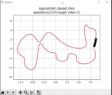
plt.title("SINGAPORE GRAND PRIX\n" + "speed[m/s]:" + str(
round(np.mean(u_lqr), 2)) +
",target index:" + str(ind))
plt.pause(0.0001)
#input()
return t, traj
def main():
# Countdown to start
print("\n*** SINGAPORE GRAND PRIX ***\n")
print("Start your engines!")
print("3.0")
sleep(1.0)
print("2.0")
sleep(1.0)
print("1.0\n")
sleep(1.0)
print("LQR + EKF steering control tracking start!!")
# Create the track waypoints
ax = [8.3,8.0, 7.2, 6.5, 6.2, 6.5, 1.5,-2.0,-3.5,-5.0,-7.9,
-6.7,-6.7,-5.2,-3.2,-1.2, 0.0, 0.2, 2.5, 2.8, 4.4, 4.5, 7.8, 8.5, 8.3]
ay = [0.7,4.3, 4.5, 5.2, 4.0, 0.7, 1.3, 3.3, 1.5, 3.0,-1.0,
-2.0,-3.0,-4.5, 1.1,-0.7,-1.0,-2.0,-2.2,-1.2,-1.5,-2.4,-2.7,-1.7,-0.1]
# These landmarks help the mobile robot localize itself
landmarks = [[4,3],
[8,2],
[-1,-4]]
# Compute the desired trajectory
desired_traj = compute_traj(ax,ay)
t, traj = closed_loop_prediction(desired_traj,landmarks)
# Display the trajectory that the mobile robot executed
if show_animation:
plt.close()
flg, _ = plt.subplots(1)
plt.plot(ax, ay, "xb", label="input")
plt.plot(desired_traj[:,0], desired_traj[:,1], "-r", label="spline")
plt.plot(traj[:,0], traj[:,1], "-g", label="tracking")
plt.grid(True)
plt.axis("equal")
plt.xlabel("x[m]")
plt.ylabel("y[m]")
plt.legend()
plt.show()
if __name__ == '__main__':
main()
sensors.py
"""
Extended Kalman Filter implementation using landmarks to localize

Implemented by Addison Sears-Collins
Date: December 10, 2020
"""
import numpy as np
import scipy.linalg as la
import math

class LandmarkDetector(object):
  """
  This class represents the sensor mounted on the robot that is used to
  to detect the location of landmarks in the environment.
  """
  def __init__(self,landmark_list):
    """
    Calculates the sensor measurements for the landmark sensor

    Input
      :param landmark_list: 2D list of landmarks [L1,L2,L3,...,LN],
                            where each row is a 2D landmark defined by
						                Li =[l_i_x,l_i_y]
                            which corresponds to its x position and y
                            position in the global coordinate frame.
    """
    # Store the x and y position of each landmark in the world
    self.landmarks = np.array(landmark_list)

    # Record the total number of landmarks
    self.N_landmarks = self.landmarks.shape[0]

    # Variable that represents landmark sensor noise (i.e. error)
    self.W = None

  def get_W(self):
    """
    This function provides the covariance matrix W which describes the noise
    that can be applied to the sensor measurements.

    Feel free to experiment with different levels of noise.

    Output
      :return: W: measurement noise matrix (4x4 matrix given two landmarks)
                  In this implementation there are two landmarks.
                  Each landmark has an x location and y location, so there are
                  4 individual sensor measurements.
    """
    # In the EKF code, we will condense this 4x4 matrix so that it is a 4x1
    # landmark sensor measurement noise vector (i.e. [x1 noise, y1 noise, x2
    # noise, y2 noise]
    if self.W is None:
      self.W = 0.0095*np.eye(2*self.N_landmarks)
    return self.W

  def measure(self,x,w=None):
    """
    Computes the landmark sensor measurements for the system.
    This will be a list of range (i.e. distance)
    and relative angles between the robot and a
    set of landmarks defined with [x,y] positions.

    Input
      :param x: The state [x_t,y_t,theta_t] of the system -> np.array with
                shape (3,). x is a 3x1 vector
      :param w: The noise (assumed Gaussian) applied to the measurement ->
                np.array with shape (2 * N_Landmarks,)
                w is a 4x1 vector
    Output
      :return: y: The resulting observation vector (4x1 in this
                  implementation because there are 2 landmarks). The
                  resulting measurement is
                  y = [h1_range_1,h1_angle_1, h2_range_2, h2_angle_2]
    """
    # Create the observation vector
    y = np.zeros(shape=(2*self.N_landmarks,))

    # Initialize state variables
    x_t = x[0]
    y_t = x[1]
    THETA_t = x[2]

    # Fill in the observation model y
    for i in range(0, self.N_landmarks):

      # Set the x and y position for landmark i
      x_l_i = self.landmarks[i][0]
      y_l_i = self.landmarks[i][1]

      # Set the noise value
      w_r = w[i*2]
      w_b = w[i*2+1]

      # Calculate the range (distance from robot to the landmark) and
			# bearing angle to the landmark
      range_i = math.sqrt(((x_t - x_l_i)**2) + ((y_t - y_l_i)**2)) + w_r
      angle_i = math.atan2(y_t - y_l_i,x_t - x_l_i) - THETA_t + w_b

      # Populate the predicted sensor observation vector
      y[i*2] = range_i
      y[i*2+1] = angle_i

    return y

  def jacobian(self,x):
    """
    Computes the first order jacobian around the state x

    Input
      :param x: The starting state (position) of the system -> np.array
                with shape (3,)

    Output
      :return: H: The resulting Jacobian matrix H for the sensor.
                  The number of rows is equal to two times the number of
                  landmarks H. 2 rows (for the range (distance) and bearing
                  to landmark measurement) x 3 columns for the number of
                  states (X, Y, THETA).

	                In other words, the number of rows is equal to the total
                  number of individual sensor measurements.
				          Since we have 2 landmarks, H will be a 4x3 matrix
                    (2 * N_Landmarks x Number of states)
    """
    # Create the Jacobian matrix H
    # For example, the first two rows of the Jacobian matrix H pertain to
    # the first landmark:
    #   dh_range/dx_t    dh_range/dy_t    dh_range/dtheta_t
    #   dh_bearing/dx_t  dh_bearing/dy_t  dh_bearing/dtheta_t
    # Note that 'bearing' and 'angle' are synonymous in this program.
    H = np.zeros(shape=(2 * self.N_landmarks, 3))

    # Extract the state
    X_t = x[0]
    Y_t = x[1]
    THETA_t = x[2]

    # Fill in H, the Jacobian matrix with the partial derivatives of the
    # observation (measurement) model h
    # Partial derivatives were calculated using an online partial derivatives
    # calculator.
    # atan2 derivatives are listed here https://en.wikipedia.org/wiki/Atan2
    for i in range(0, self.N_landmarks):

      # Set the x and y position for landmark i
      x_l_i = self.landmarks[i][0]
      y_l_i = self.landmarks[i][1]

      dh_range_dx_t = (X_t-x_l_i) / math.sqrt((X_t-x_l_i)**2 + (Y_t-y_l_i)**2)
      H[i*2][0] = dh_range_dx_t

      dh_range_dy_t = (Y_t-y_l_i) / math.sqrt((X_t-x_l_i)**2 + (Y_t-y_l_i)**2)
      H[i*2][1] = dh_range_dy_t

      dh_range_dtheta_t = 0
      H[i*2][2] = dh_range_dtheta_t

      dh_bearing_dx_t = -(Y_t-y_l_i) / ((X_t-x_l_i)**2 + (Y_t-y_l_i)**2)
      H[i*2+1][0] = dh_bearing_dx_t

      dh_bearing_dy_t = (X_t-x_l_i) / ((X_t-x_l_i)**2 + (Y_t-y_l_i)**2)
      H[i*2+1][1] = dh_bearing_dy_t

      dh_bearing_dtheta_t = -1.0
      H[i*2+1][2] = dh_bearing_dtheta_t

    return H

def EKF(DiffDrive,Sensor,y,x_hat,sigma,u,dt,V=None,W=None):
    """
    Some of these matrices will be non-square or singular. Utilize the
    pseudo-inverse function la.pinv instead of inv to avoid these errors.

    Input
      :param DiffDrive: The DifferentialDrive object defined in kinematics.py
      :param Sensor: The Landmark Sensor object defined in this class
      :param y: The observation vector (4x1 in this implementation because
                there are 2 landmarks). The measurement is
                y = [h1_range_1,h1_angle_1, h2_range_2, h2_angle_2]
      :param x_hat: The starting estimate of the state at time t ->
                    np.array with shape (3,)
                    (X_t, Y_t, THETA_t)
      :param sigma: The state covariance matrix at time t -> np.array with
                    shape (3,1) initially, then 3x3
      :param u: The input to the system at time t -> np.array with shape (2,1)
                These are the control inputs to the system.
                [left wheel rotational velocity, right wheel rotational
                velocity]
      :param dt: timestep size delta t
      :param V: The state noise covariance matrix  -> np.array with shape (3,3)
      :param W: The measurment noise covariance matrix -> np.array with shape
                (2*N_Landmarks,2*N_Landmarks)
                4x4 matrix

    Output
      :return: x_hat_2: The estimate of the state at time t+1
                        [X_t+1, Y_t+1, THETA_t+1]
      :return: sigma_est: The new covariance matrix at time t+1 (3x3 matrix)

    """
    V = DiffDrive.get_V() # 3x3 matrix for the state noise
    W = Sensor.get_W() # 4x4 matrix for the measurement noise

    ## Generate noise
    # v = process noise, w = measurement noise
    v = np.random.multivariate_normal(np.zeros(V.shape[0]),V) # 3x1 vector
    w = np.random.multivariate_normal(np.zeros(W.shape[0]),W) # 4x1 vector

	##### Prediction Step #####

    # Predict the state estimate based on the previous state and the
    # control input
    # x_predicted is a 3x1 vector (X_t+1, Y_t+1, THETA_t+1)
    x_predicted = DiffDrive.forward(x_hat,u,v,dt)

    # Calculate the A and B matrices
    A, B = DiffDrive.linearize(x=x_hat)

    # Predict the covariance estimate based on the
    # previous covariance and some noise
    # A and V are 3x3 matrices
    sigma_3by3 = None
    if (sigma.size == 3):
      sigma_3by3 = sigma * np.eye(3)
    else:
      sigma_3by3 = sigma

    sigma_new = A @ sigma_3by3 @ A.T + V

    ##### Correction Step #####

    # Get H, the 4x3 Jacobian matrix for the sensor
    H = Sensor.jacobian(x_hat)

    # Calculate the observation model
    # y_predicted is a 4x1 vector
    y_predicted = Sensor.measure(x_predicted, w)

    # Measurement residual (delta_y is a 4x1 vector)
    delta_y = y - y_predicted

    # Residual covariance
    # 4x3 @ 3x3 @ 3x4 -> 4x4 matrix
    S = H @ sigma_new @ H.T + W

    # Compute the Kalman gain
    # The Kalman gain indicates how certain you are about
    # the observations with respect to the motion
    # 3x3 @ 3x4 @ 4x4 -> 3x4
    K = sigma_new @ H.T @ la.pinv(S)

    # Update the state estimate
    # 3x1 + (3x4 @ 4x1 -> 3x1)
    x_hat_2 = x_predicted + (K @ delta_y)

    # Update the covariance estimate
    # 3x3 - (3x4 @ 4x3) @ 3x3
    sigma_est = sigma_new - (K @ H @ sigma_new)

    return x_hat_2 , sigma_est
utils.py
"""
Program: utils.py
This program helps calculate the waypoints along the racetrack
that the robot needs to follow.

Modified from code developed by Atsushi Sakai
Source: https://github.com/AtsushiSakai/PythonRobotics
"""
import numpy as np
import math
import cubic_spline_planner

def pi_2_pi(angle):
    return (angle + math.pi) % (2*math.pi) - math.pi

def compute_traj(ax,ay):
    cx, cy, cyaw, ck, s = cubic_spline_planner.calc_spline_course(
        ax, ay, ds=0.1)
    target_speed = 1  # simulation parameter km/h -> m/s
    sp = calc_speed_profile(cx, cy, cyaw, target_speed)

    desired_traj = np.array([cx,cy,cyaw,sp]).T
    return desired_traj

def calc_nearest_index(state, traj):
    cx = traj[:,0]
    cy = traj[:,1]
    cyaw = traj[:,2]
    dx = [state[0] - icx for icx in cx]
    dy = [state[1] - icy for icy in cy]

    d = [idx ** 2 + idy ** 2 for (idx, idy) in zip(dx, dy)]

    mind = min(d)

    ind = d.index(mind)

    mind = math.sqrt(mind)

    dxl = cx[ind] - state[0]
    dyl = cy[ind] - state[1]

    angle = pi_2_pi(cyaw[ind] - math.atan2(dyl, dxl))
    if angle < 0:
        mind *= -1

    return ind, mind


def calc_speed_profile(cx, cy, cyaw, target_speed):
    speed_profile = [target_speed] * len(cx)

    direction = 1.0

    # Set stop point
    for i in range(len(cx) - 1):
        dyaw = abs(cyaw[i + 1] - cyaw[i])
        switch = math.pi / 4.0 <= dyaw < math.pi / 2.0

        if switch:
            direction *= -1

        if direction != 1.0:
            speed_profile[i] = - target_speed
        else:
            speed_profile[i] = target_speed

        if switch:
            speed_profile[i] = 0.0

    speed_profile[-1] = 0.0

    return speed_profile
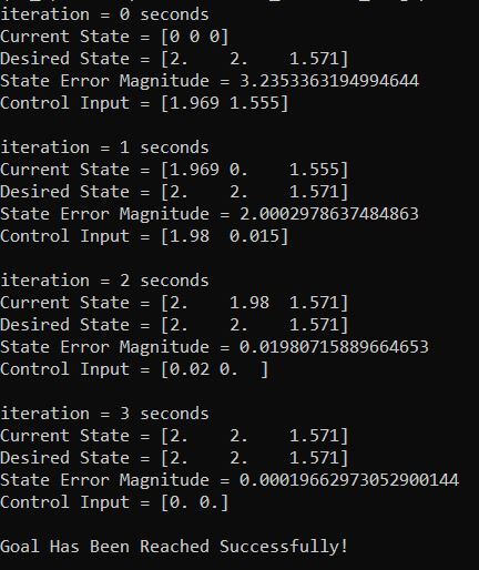
To run the code, navigate to the directory and run the lqr_ekf_control.py program. I’m using Anaconda to run my Python programs, so I’ll type:
python lqr_ekf_control.py
Keep building!