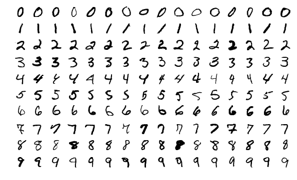
In this tutorial, we will build a convolutional neural network that can classify handwritten digits (i.e. 0 through 9). We will train and test our neural networking using the MNIST data set, a large data set of handwritten digits that is often used as a first project for people who are getting started in deep learning for computer vision.
If you want to use GPU support for your TensorFlow installation, you will need to follow these steps. If you have trouble following those steps, you can follow these steps (note that the steps change quite frequently, but the overall process remains relatively the same).
This post can also help you get your system setup, including your virtual environment in Anaconda (if you decide to go this route).
Directions
Open up a new Python program (in your favorite text editor or Python IDE), and write the following code. I’m going to name the program mnist_handwritten_digits.py.
Here is the code. Don’t be afraid of how long the code is. All you need to do is copy the code and paste it in a file. I included a lot of comments. I’ll explain each piece of the code in detail in a second.
# Project: Detect Handwritten Digits Using the MNIST Data Set
# Author: Addison Sears-Collins
# Date created: January 4, 2021
import tensorflow as tf # Machine learning library
from tensorflow import keras # Library for neural networks
from tensorflow.keras.datasets import mnist # MNIST data set
from tensorflow.keras.layers import Conv2D, Dense, Flatten, MaxPooling2D
from tensorflow.keras.optimizers import Adam
from tensorflow.keras.losses import categorical_crossentropy
import numpy as np
from time import time
import matplotlib.pyplot as plt
num_classes = 10 # Number of distinct labels
def generate_neural_network(x_train):
"""
Create a convolutional neural network.
:x_train: Training images of handwritten digits (grayscale)
:return: Neural network
"""
model = keras.Sequential()
# Add a convolutional layer to the neural network
model.add(Conv2D(filters=6, kernel_size=(
5, 5), activation='relu', padding='same', input_shape=x_train.shape[
1:]))
model.add(MaxPooling2D()) # subsampling using max pooling
# Add a convolutional layer to the neural network
model.add(Conv2D(filters=16, kernel_size=(5, 5), activation='relu'))
model.add(MaxPooling2D())
# Add the dense layers
model.add(Flatten())
model.add(Dense(units=120, activation='relu'))
model.add(Dense(units=84, activation='relu'))
# Softmax transforms the prediction into a probability
# The highest probability corresponds to the category of the image (i.e. 0-9)
model.add(Dense(units=num_classes, activation='softmax'))
return model
def tf_and_gpu_ok():
"""
Test if TensorFlow and GPU support are working properly.
"""
# Test code to see if Tensorflow is installed properly
print("Tensorflow:", tf.__version__)
print("Tensorflow Git:", tf.version.GIT_VERSION)
# See if you can use the GPU on your computer
print("CUDA ON" if tf.test.is_built_with_cuda() else "CUDA OFF")
print("GPU ON" if tf.test.is_gpu_available() else "GPU OFF")
def main():
# Uncomment to check if everything is working properly
#tf_and_gpu_ok()
# Load the MNIST data set and make sure the training and testing
# data are four dimensions (which is what Keras needs)
(x_train, y_train), (x_test, y_test) = mnist.load_data()
x_train = np.reshape(x_train, np.append(x_train.shape, (1)))
x_test = np.reshape(x_test, np.append(x_test.shape, (1)))
# Uncomment to display the dimensions of the training data set and the
# testing data set
#print('x_train', x_train.shape, ' --- x_test', x_test.shape)
#print('y_train', y_train.shape, ' --- y_test', y_test.shape)
# Normalize image intensity values to a range between 0 and 1 (from 0-255)
x_train = x_train.astype('float32')
x_test = x_test.astype('float32')
x_train = x_train / 255
x_test = x_test / 255
# Uncomment to display the first 3 labels
#print('First 3 labels for train set:', y_train[0], y_train[1], y_train[2])
#print('First 3 labels for testing set:', y_test[0], y_test[1], y_test[2])
# Perform one-hot encoding
y_train = keras.utils.to_categorical(y_train, num_classes)
y_test = keras.utils.to_categorical(y_test, num_classes)
# Create the neural network
model = generate_neural_network(x_train)
# Uncomment to print the summary statistics of the neural network
#print(model.summary())
# Configure the neural network
model.compile(loss=categorical_crossentropy, optimizer=Adam(), metrics=['accuracy'])
start = time()
history = model.fit(x_train, y_train, batch_size=16, epochs=5, validation_data=(x_test, y_test), shuffle=True)
training_time = time() - start
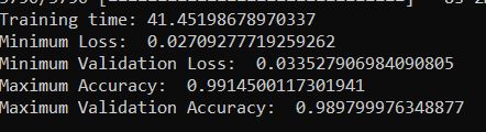
print(f'Training time: {training_time}')
# A measure of how well the neural network learned the training data
# The lower, the better
print("Minimum Loss: ", min(history.history['loss']))
# A measure of how well the neural network did on the validation data set
# The lower, the better
print("Minimum Validation Loss: ", min(history.history['val_loss']))
# Maximum percentage of correct predictions on the training data
# The higher, the better
print("Maximum Accuracy: ", max(history.history['accuracy']))
# Maximum percentage of correct predictions on the validation data
# The higher, the better
print("Maximum Validation Accuracy: ", max(history.history['val_accuracy']))
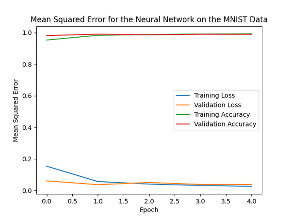
# Plot the key statistics
plt.plot(history.history['loss'])
plt.plot(history.history['val_loss'])
plt.plot(history.history['accuracy'])
plt.plot(history.history['val_accuracy'])
plt.title("Mean Squared Error for the Neural Network on the MNIST Data")
plt.ylabel("Mean Squared Error")
plt.xlabel("Epoch")
plt.legend(['Training Loss', 'Validation Loss', 'Training Accuracy',
'Validation Accuracy'], loc='center right')
plt.show() # Press Q to close the graph
# Save the neural network in Hierarchical Data Format version 5 (HDF5) format
model.save('mnist_nnet.h5')
# Import the saved model
model = keras.models.load_model('mnist_nnet.h5')
print("\n\nNeural network has loaded successfully...\n")
main()
Code Walkthrough
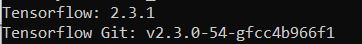
The tf_and_gpu_ok() method is used to check if:
TensorFlow is installed properly.
TensorFlow is able to use the GPU (Graphic Processing Unit) on your computer. The GPU on your computer will help speed up the training of your neural network.
If you see the output below when you run the mnist_handwritten_digits.py program…
python mnist_handwritten_digits.py
…the software is installed correctly.
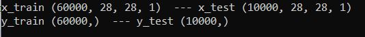
The next piece of code in main displays the dimensions of x_train and y_train. You can see from the output that we train the neural network on 60,000 grayscale images that are 28×28 pixels in size and test the data set on 10,000 grayscale images that are 28×28 pixels in size. Each image contains a handwritten number from 0-9.
At this stage, the intensity for all of the images in the sample ranges from 0-255 (i.e. grayscale). To improve the performance of the neural network, it is helpful to normalize the image intensities to values between 0 and 1. To do this, we need to take the intensity values for each image and divide by the largest value (i.e. 255).
At this stage, we have 10 different labels: 0, 1, 2, 3, 4, 5, 6, 7, 8, 9. These labels represent the 10 different categories (i.e. values) that the handwritten digits could possibly be. To enable the neural network to make better predictions, we need to convert this categorical data into a vector format of just 0s and 1s using a technique known as one-hot encoding.
For each of the 10 possible label values, you get a 10-element vector where only one element is hot (i.e. 1), and the rest of the elements are cold (i.e. 0).
For example, here is the one-hot encoding for the label possibilities in this project:
0 -> 1 0 0 0 0 0 0 0 0 0
1 -> 0 1 0 0 0 0 0 0 0 0
2 -> 0 0 1 0 0 0 0 0 0 0
3 -> 0 0 0 1 0 0 0 0 0 0
4 -> 0 0 0 0 1 0 0 0 0 0
5 -> 0 0 0 0 0 1 0 0 0 0
6 -> 0 0 0 0 0 0 1 0 0 0
7 -> 0 0 0 0 0 0 0 1 0 0
8 -> 0 0 0 0 0 0 0 0 1 0
9 -> 0 0 0 0 0 0 0 0 0 1
Now, we need to generate the neural network. I created a method named generate_neural_network to do just that. If there is something you don’t understand in the code, consult the reference for Keras.
If you want to understand how neural networks make predictions, check out this post.
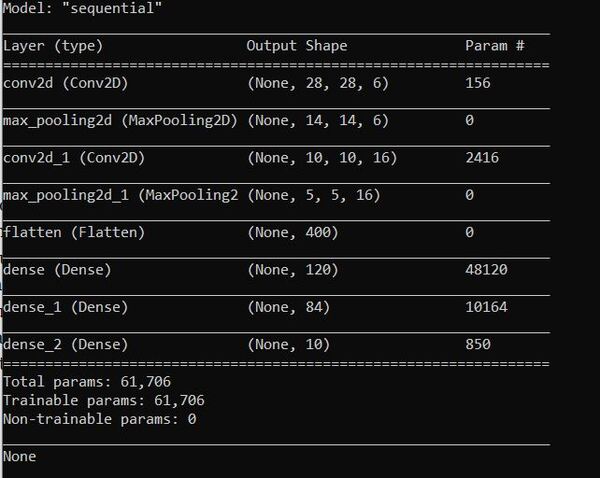
Here is what you will see for the summary statistics:
You can see that the neural network has 61,706 parameters. This number is considerably more than the 4,865 parameters used when we used a deep neural network to predict vehicle fuel economy because we are dealing with images rather than just numbers. As the saying goes, “A picture is worth 1,000 words.”
Now that we have constructed our neural network, we need to train it so that it can be able to make predictions (i.e. convert handwritten numbers into digits 0-9).
We need to feed our network the training samples that consist of the handwritten digits and the corresponding truth (i.e. the labels 0-9). Then we need to train the model and store the data into the history object. If you run the program and hit issues with the version of cuDNN, go to the Anaconda terminal, and type:
conda install -c anaconda cudnn
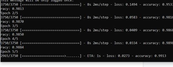
When you run the program, you will see that the accuracy statistics are around 99%.
You should see output on the terminal similar to this graphic when you train the neural network.
At the end of main, I saved our neural network in Hierarchical Data Format version 5 (HDF5) format. I then added some other code to show you how to load the model if you want to do that at a later date.
That’s it! You now know how to build a neural network to accurately classify handwritten digits.
Last week, I built a mobile robot in Gazebo that uses ROS2 for message passing. I wanted the robot to go to predefined goal coordinates inside a maze. In order to do that, I needed to create a Publisher node that published the points to a topic.
Here is the ROS2 node code (in Python) that publishes a list of target coordinates (i.e. waypoints) for the mobile robot to go to. Feel free to use this code for your ROS2 projects:
''' ####################
    Publish (x,y) coordinate goals for a differential drive robot in a
    Gazebo maze.
    ==================================
    Author: Addison Sears-Collins
    Date: November 21, 2020
    #################### '''

import rclpy # Import the ROS client library for Python
from rclpy.node import Node # Enables the use of rclpy's Node class
from std_msgs.msg import Float64MultiArray # Enable use of std_msgs/Float64MultiArray message

class GoalPublisher(Node):
  """
  Create a GoalPublisher class, which is a subclass of the Node class.
  The class publishes the goal positions (x,y) for a mobile robot in a Gazebo maze world.
  """

  def __init__(self):
    """
    Class constructor to set up the node
    """

    # Initiate the Node class's constructor and give it a name
    super().__init__('goal_publisher')

    # Create publisher(s)
    self.publisher_goal_x_values = self.create_publisher(Float64MultiArray, '/goal_x_values', 10)
    self.publisher_goal_y_values = self.create_publisher(Float64MultiArray, '/goal_y_values', 10)

    # Call the callback functions every 0.5 seconds
    timer_period = 0.5
    self.timer1 = self.create_timer(timer_period, self.get_x_values)
    self.timer2 = self.create_timer(timer_period, self.get_y_values)

    # Initialize a counter variable
    self.i = 0
    self.j = 0

    # List the goal destinations
    # We create a list of the (x,y) coordinate goals
    self.goal_x_coordinates = [ 0.0, 3.0, 0.0, -1.5, -1.5,  4.5, 0.0]
    self.goal_y_coordinates = [-4.0, 1.0, 1.5,  1.0, -3.0, -4.0, 0.0]

  def get_x_values(self):
    """
    Callback function.
    """
    msg = Float64MultiArray()
    msg.data = self.goal_x_coordinates

    # Publish the x coordinates to the topic
    self.publisher_goal_x_values.publish(msg)

    # Increment counter variable
    self.i += 1

  def get_y_values(self):
    """
    Callback function.
    """
    msg = Float64MultiArray()
    msg.data = self.goal_y_coordinates

    # Publish the y coordinates to the topic
    self.publisher_goal_y_values.publish(msg)

    # Increment counter variable
    self.j += 1

def main(args=None):

  # Initialize the rclpy library
  rclpy.init(args=args)

  # Create the node
  goal_publisher = GoalPublisher()

  # Spin the node so the callback function is called.
  # Publish any pending messages to the topics.
  rclpy.spin(goal_publisher)

  # Destroy the node explicitly
  # (optional - otherwise it will be done automatically
  # when the garbage collector destroys the node object)
  goal_publisher.destroy_node()

  # Shutdown the ROS client library for Python
  rclpy.shutdown()

if __name__ == '__main__':
  main()
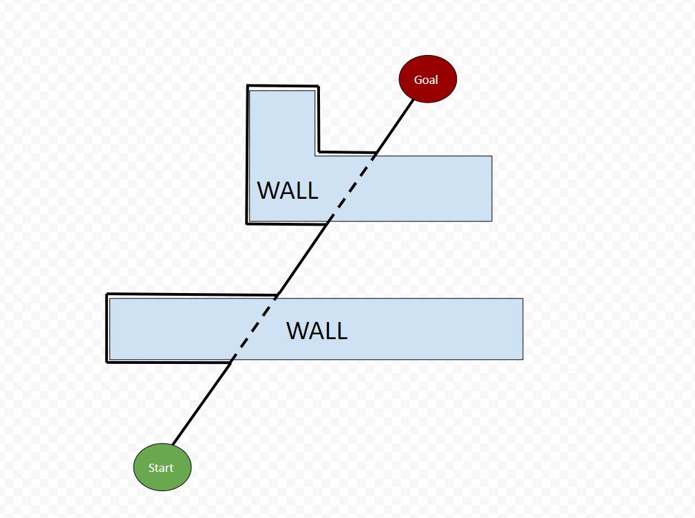
In this tutorial, we will learn about the Bug2 algorithm for robot motion planning. The Bug2 algorithm is used when you have a mobile robot:
With a known starting location
With a known goal location
Inside an unexplored environment
Contains a distance sensor that can detect the distances to objects and walls in the environment (e.g. like an ultrasonic sensor or a laser distance sensor.)
Contains an encoder that the robot can use to estimate how far the robot has traveled from the starting location.
Here is a video of a simulated robot I developed in Gazebo and ROS2 that uses the Bug2 algorithm to move from a starting point to a goal point, avoiding walls along the way.
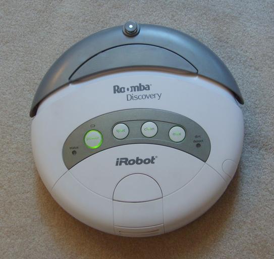
Real-World Applications
Imagine an automatic vacuum cleaner like the one below. It vacuums a room and then needs to move autonomously to another room so that it can clean that room. Along the way, the robot must avoid bumping into walls.
Algorithm Description
On a high level, the Bug2 algorithm has two main modes:
Go to Goal Mode: Move from the current location towards the goal (x,y) coordinate.
Wall Following Mode: Move along a wall.
Here is pseudocode for the algorithm:
1. Calculate a start-goal line. The start-goal line is an imaginary line that connects the starting position to the goal position.
2. While Not at the Goal
Move towards the goal along the start-goal line.
If a wall is encountered:
Remember the location where the wall was first encountered. This is the “hit point.”
Follow the wall until you encounter the start-goal line. This point is known as the “leave point.”
If the leave point is closer to the goal than the hit point, leave the wall, and move towards the goal again.
Otherwise, continue following the wall.
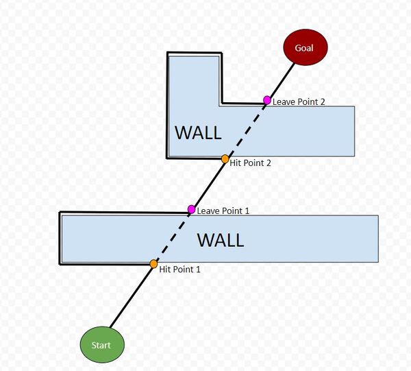
That’s the algorithm. In the image below, I have labeled the hit points and leave points.
Python Implementation (ROS2)
The robot you see in the video at the beginning of this tutorial has a laser distance scanner mounted on top of it that enables it to detect distances from 0 degrees (right side of the robot) to 180 degrees (left side of the robot). It is using three Python functions, bug2, follow_wall, and go_to_goal.
Below is my complete code. It runs in ROS2 Foxy Fitzroy and Gazebo and makes use of the Differential Drive plugin.
Since we’re just focusing on the algorithms in this post, I won’t go into the details of how I created the robot, built the simulated maze, and created publisher and subscriber nodes for the goal locations, robot pose, and laser distance sensor information (I might cover this in a future post).
Don’t be intimidated by the code. It is long but well-commented. Go through each piece and function one step at a time. Focus only on the following three methods:
go_to_goal(self)method
follow_wall(self) method
bug2(self) method
Those three methods encapsulate the implementation of Bug2.
I created descriptive variable names so that you can compare the code to the pseudocode I wrote earlier in this tutorial.
# Author: Addison Sears-Collins
# Date: December 17, 2020
# ROS Version: ROS 2 Foxy Fitzroy

############## IMPORT LIBRARIES #################
# Python math library
import math

# ROS client library for Python
import rclpy

# Enables pauses in the execution of code
from time import sleep

# Used to create nodes
from rclpy.node import Node

# Enables the use of the string message type
from std_msgs.msg import String

# Twist is linear and angular velocity
from geometry_msgs.msg import Twist

# Handles LaserScan messages to sense distance to obstacles (i.e. walls)
from sensor_msgs.msg import LaserScan

# Handle Pose messages
from geometry_msgs.msg import Pose

# Handle float64 arrays
from std_msgs.msg import Float64MultiArray

# Handles quality of service for LaserScan data
from rclpy.qos import qos_profile_sensor_data

# Scientific computing library
import numpy as np

class PlaceholderController(Node):
	"""
	Create a Placeholder Controller class, which is a subclass of the Node
	class for ROS2.
	"""

	def __init__(self):
		"""
		Class constructor to set up the node
		"""
		####### INITIALIZE ROS PUBLISHERS AND SUBSCRIBERS##############
		# Initiate the Node class's constructor and give it a name
		super().__init__('PlaceholderController')

		# Create a subscriber
		# This node subscribes to messages of type Float64MultiArray
		# over a topic named: /en613/state_est
		# The message represents the current estimated state:
		#   [x, y, yaw]
		# The callback function is called as soon as a message
		# is received.
		# The maximum number of queued messages is 10.
		self.subscription = self.create_subscription(
			Float64MultiArray,
			'/en613/state_est',
			self.state_estimate_callback,
			10)
		self.subscription  # prevent unused variable warning

		# Create a subscriber
		# This node subscribes to messages of type
		# sensor_msgs/LaserScan
		self.scan_subscriber = self.create_subscription(
			LaserScan,
			'/en613/scan',
			self.scan_callback,
			qos_profile=qos_profile_sensor_data)

		# Create a subscriber
		# This node subscribes to messages of type geometry_msgs/Pose
		# over a topic named: /en613/goal
		# The message represents the the goal position.
		# The callback function is called as soon as a message
		# is received.
		# The maximum number of queued messages is 10.
		self.subscription_goal_pose = self.create_subscription(
			Pose,
			'/en613/goal',
			self.pose_received,
			10)

		# Create a publisher
		# This node publishes the desired linear and angular velocity
		# of the robot (in the robot chassis coordinate frame) to the
		# /en613/cmd_vel topic. Using the diff_drive
		# plugin enables the basic_robot model to read this
		# /end613/cmd_vel topic and execute the motion accordingly.
		self.publisher_ = self.create_publisher(
			Twist,
			'/en613/cmd_vel',
			10)

		# Initialize the LaserScan sensor readings to some large value
		# Values are in meters.
		self.left_dist = 999999.9 # Left
		self.leftfront_dist = 999999.9 # Left-front
		self.front_dist = 999999.9 # Front
		self.rightfront_dist = 999999.9 # Right-front
		self.right_dist = 999999.9 # Right

		################### ROBOT CONTROL PARAMETERS ##################

		# Maximum forward speed of the robot in meters per second
		# Any faster than this and the robot risks falling over.
		self.forward_speed = 0.035

		# Current position and orientation of the robot in the global
		# reference frame
		self.current_x = 0.0
		self.current_y = 0.0
		self.current_yaw = 0.0

		# By changing the value of self.robot_mode, you can alter what
		# the robot will do when the program is launched.
		# 	"obstacle avoidance mode": Robot will avoid obstacles
		#  	"go to goal mode": Robot will head to an x,y coordinate
		# 	"wall following mode": Robot will follow a wall
		self.robot_mode = "go to goal mode"

		############# OBSTACLE AVOIDANCE MODE PARAMETERS ##############

		# Obstacle detection distance threshold
		self.dist_thresh_obs = 0.25 # in meters

		# Maximum left-turning speed
		self.turning_speed = 0.25 # rad/s

		############# GO TO GOAL MODE PARAMETERS ######################
		# Finite states for the go to goal mode
		# 	"adjust heading": Orient towards a goal x, y coordinate
		# 	"go straight": Go straight towards goal x, y coordinate
		# 	"goal achieved": Reached goal x, y coordinate
		self.go_to_goal_state = "adjust heading"

		# List the goal destinations
		# We create a list of the (x,y) coordinate goals
		self.goal_x_coordinates = False # [ 0.0, 3.0, 0.0, -1.5, -1.5,  4.5, 0.0]
		self.goal_y_coordinates = False # [-4.0, 1.0, 1.5,  1.0, -3.0, -4.0, 0.0]

		# Keep track of which goal we're headed towards
		self.goal_idx = 0

		# Keep track of when we've reached the end of the goal list
		self.goal_max_idx =  None # len(self.goal_x_coordinates) - 1

		# +/- 2.0 degrees of precision
		self.yaw_precision = 2.0 * (math.pi / 180)

		# How quickly we need to turn when we need to make a heading
		# adjustment (rad/s)
		self.turning_speed_yaw_adjustment = 0.0625

		# Need to get within +/- 0.2 meter (20 cm) of (x,y) goal
		self.dist_precision = 0.2

		############# WALL FOLLOWING MODE PARAMETERS ##################
		# Finite states for the wall following mode
		# 	"turn left": Robot turns towards the left
		#	"search for wall": Robot tries to locate the wall
		# 	"follow wall": Robot moves parallel to the wall
		self.wall_following_state = "turn left"

		# Set turning speeds (to the left) in rad/s
		# These values were determined by trial and error.
		self.turning_speed_wf_fast = 1.0  # Fast turn
		self.turning_speed_wf_slow = 0.125 # Slow turn

		# Wall following distance threshold.
		# We want to try to keep within this distance from the wall.
		self.dist_thresh_wf = 0.45 # in meters

		# We don't want to get too close to the wall though.
		self.dist_too_close_to_wall = 0.15 # in meters

		################### BUG2 PARAMETERS ###########################

		# Bug2 Algorithm Switch
		# Can turn "ON" or "OFF" depending on if you want to run Bug2
		# Motion Planning Algorithm
		self.bug2_switch = "ON"

		# Start-Goal Line Calculated?
		self.start_goal_line_calculated = False

		# Start-Goal Line Parameters
		self.start_goal_line_slope_m = 0
		self.start_goal_line_y_intercept = 0
		self.start_goal_line_xstart = 0
		self.start_goal_line_xgoal = 0
		self.start_goal_line_ystart = 0
		self.start_goal_line_ygoal = 0

		# Anything less than this distance means we have encountered
		# a wall. Value determined through trial and error.
		self.dist_thresh_bug2 = 0.15

		# Leave point must be within +/- 0.1m of the start-goal line
		# in order to go from wall following mode to go to goal mode
		self.distance_to_start_goal_line_precision = 0.1

		# Used to record the (x,y) coordinate where the robot hit
		# a wall.
		self.hit_point_x = 0
		self.hit_point_y = 0

		# Distance between the hit point and the goal in meters
		self.distance_to_goal_from_hit_point = 0.0

		# Used to record the (x,y) coordinate where the robot left
		# a wall.
		self.leave_point_x = 0
		self.leave_point_y = 0

		# Distance between the leave point and the goal in meters
		self.distance_to_goal_from_leave_point = 0.0

		# The hit point and leave point must be far enough
		# apart to change state from wall following to go to goal
		# This value helps prevent the robot from getting stuck and
		# rotating in endless circles.
		# This distance was determined through trial and error.
		self.leave_point_to_hit_point_diff = 0.25 # in meters

	def pose_received(self,msg):
		"""
		Populate the pose.
		"""
		self.goal_x_coordinates = [msg.position.x]
		self.goal_y_coordinates = [msg.position.y]
		self.goal_max_idx = len(self.goal_x_coordinates) - 1

	def scan_callback(self, msg):
		"""
		This method gets called every time a LaserScan message is
		received on the /en613/scan ROS topic
		"""
		# Read the laser scan data that indicates distances
		# to obstacles (e.g. wall) in meters and extract
		# 5 distinct laser readings to work with.
		# Each reading is separated by 45 degrees.
		# Assumes 181 laser readings, separated by 1 degree.
		# (e.g. -90 degrees to 90 degrees....0 to 180 degrees)
		self.left_dist = msg.ranges[180]
		self.leftfront_dist = msg.ranges[135]
		self.front_dist = msg.ranges[90]
		self.rightfront_dist = msg.ranges[45]
		self.right_dist = msg.ranges[0]

		# The total number of laser rays. Used for testing.
		#number_of_laser_rays = str(len(msg.ranges))

		# Print the distance values (in meters) for testing
		#self.get_logger().info('L:%f LF:%f F:%f RF:%f R:%f' % (
		#	self.left_dist,
		#	self.leftfront_dist,
		#	self.front_dist,
		#	self.rightfront_dist,
		#	self.right_dist))

		if self.robot_mode == "obstacle avoidance mode":
			self.avoid_obstacles()

	def state_estimate_callback(self, msg):
		"""
		Extract the position and orientation data.
		This callback is called each time
		a new message is received on the '/en613/state_est' topic
		"""
		# Update the current estimated state in the global reference frame
		curr_state = msg.data
		self.current_x = curr_state[0]
		self.current_y = curr_state[1]
		self.current_yaw = curr_state[2]

		# Wait until we have received some goal destinations.
		if self.goal_x_coordinates == False and self.goal_y_coordinates == False:
			return

		# Print the pose of the robot
		# Used for testing
		#self.get_logger().info('X:%f Y:%f YAW:%f' % (
		#	self.current_x,
		#	self.current_y,
		#	np.rad2deg(self.current_yaw)))  # Goes from -pi to pi

		# See if the Bug2 algorithm is activated. If yes, call bug2()
		if self.bug2_switch == "ON":
			self.bug2()
		else:

			if self.robot_mode == "go to goal mode":
				self.go_to_goal()
			elif self.robot_mode == "wall following mode":
				self.follow_wall()
			else:
				pass # Do nothing

	def avoid_obstacles(self):
		"""
		Wander around the maze and avoid obstacles.
		"""
		# Create a Twist message and initialize all the values
		# for the linear and angular velocities
		msg = Twist()
		msg.linear.x = 0.0
		msg.linear.y = 0.0
		msg.linear.z = 0.0
		msg.angular.x = 0.0
		msg.angular.y = 0.0
		msg.angular.z = 0.0

		# Logic for avoiding obstacles (e.g. walls)
		# >d means no obstacle detected by that laser beam
		# <d means an obstacle was detected by that laser beam
		d = self.dist_thresh_obs
		if   self.leftfront_dist > d and self.front_dist > d and self.rightfront_dist > d:
			msg.linear.x = self.forward_speed # Go straight forward
		elif self.leftfront_dist > d and self.front_dist < d and self.rightfront_dist > d:
			msg.angular.z = self.turning_speed  # Turn left
		elif self.leftfront_dist > d and self.front_dist > d and self.rightfront_dist < d:
			msg.angular.z = self.turning_speed
		elif self.leftfront_dist < d and self.front_dist > d and self.rightfront_dist > d:
			msg.angular.z = -self.turning_speed # Turn right
		elif self.leftfront_dist > d and self.front_dist < d and self.rightfront_dist < d:
			msg.angular.z = self.turning_speed
		elif self.leftfront_dist < d and self.front_dist < d and self.rightfront_dist > d:
			msg.angular.z = -self.turning_speed
		elif self.leftfront_dist < d and self.front_dist < d and self.rightfront_dist < d:
			msg.angular.z = self.turning_speed
		elif self.leftfront_dist < d and self.front_dist > d and self.rightfront_dist < d:
			msg.linear.x = self.forward_speed
		else:
			pass

		# Send the velocity commands to the robot by publishing
		# to the topic
		self.publisher_.publish(msg)

	def go_to_goal(self):
		"""
		This code drives the robot towards to the goal destination
		"""
		# Create a geometry_msgs/Twist message
		msg = Twist()
		msg.linear.x = 0.0
		msg.linear.y = 0.0
		msg.linear.z = 0.0
		msg.angular.x = 0.0
		msg.angular.y = 0.0
		msg.angular.z = 0.0

		# If Bug2 algorithm is activated
		if self.bug2_switch == "ON":

			# If the wall is in the way
			d = self.dist_thresh_bug2
			if (	self.leftfront_dist < d or
				self.front_dist < d or
				self.rightfront_dist < d):

				# Change the mode to wall following mode.
				self.robot_mode = "wall following mode"

				# Record the hit point
				self.hit_point_x = self.current_x
				self.hit_point_y = self.current_y

				# Record the distance to the goal from the
				# hit point
				self.distance_to_goal_from_hit_point = (
					math.sqrt((
					pow(self.goal_x_coordinates[self.goal_idx] - self.hit_point_x, 2)) + (
					pow(self.goal_y_coordinates[self.goal_idx] - self.hit_point_y, 2))))

				# Make a hard left to begin following wall
				msg.angular.z = self.turning_speed_wf_fast

				# Send command to the robot
				self.publisher_.publish(msg)

				# Exit this function
				return

		# Fix the heading
		if (self.go_to_goal_state == "adjust heading"):

			# Calculate the desired heading based on the current position
			# and the desired position
			desired_yaw = math.atan2(
					self.goal_y_coordinates[self.goal_idx] - self.current_y,
					self.goal_x_coordinates[self.goal_idx] - self.current_x)

			# How far off is the current heading in radians?
			yaw_error = desired_yaw - self.current_yaw

			# Adjust heading if heading is not good enough
			if math.fabs(yaw_error) > self.yaw_precision:

				if yaw_error > 0:
					# Turn left (counterclockwise)
					msg.angular.z = self.turning_speed_yaw_adjustment
				else:
					# Turn right (clockwise)
					msg.angular.z = -self.turning_speed_yaw_adjustment

				# Command the robot to adjust the heading
				self.publisher_.publish(msg)

			# Change the state if the heading is good enough
			else:
				# Change the state
				self.go_to_goal_state = "go straight"

				# Command the robot to stop turning
				self.publisher_.publish(msg)

		# Go straight
		elif (self.go_to_goal_state == "go straight"):

			position_error = math.sqrt(
						pow(
						self.goal_x_coordinates[self.goal_idx] - self.current_x, 2)
						+ pow(
						self.goal_y_coordinates[self.goal_idx] - self.current_y, 2))


			# If we are still too far away from the goal
			if position_error > self.dist_precision:

				# Move straight ahead
				msg.linear.x = self.forward_speed

				# Command the robot to move
				self.publisher_.publish(msg)

				# Check our heading
				desired_yaw = math.atan2(
					self.goal_y_coordinates[self.goal_idx] - self.current_y,
					self.goal_x_coordinates[self.goal_idx] - self.current_x)

				# How far off is the heading?
				yaw_error = desired_yaw - self.current_yaw

				# Check the heading and change the state if there is too much heading error
				if math.fabs(yaw_error) > self.yaw_precision:

					# Change the state
					self.go_to_goal_state = "adjust heading"

			# We reached our goal. Change the state.
			else:
				# Change the state
				self.go_to_goal_state = "goal achieved"

				# Command the robot to stop
				self.publisher_.publish(msg)

		# Goal achieved
		elif (self.go_to_goal_state == "goal achieved"):

			self.get_logger().info('Goal achieved! X:%f Y:%f' % (
				self.goal_x_coordinates[self.goal_idx],
				self.goal_y_coordinates[self.goal_idx]))

			# Get the next goal
			self.goal_idx = self.goal_idx + 1

			# Do we have any more goals left?
			# If we have no more goals left, just stop
			if (self.goal_idx > self.goal_max_idx):
				self.get_logger().info('Congratulations! All goals have been achieved.')
				while True:
					pass

			# Let's achieve our next goal
			else:
				# Change the state
				self.go_to_goal_state = "adjust heading"

			# We need to recalculate the start-goal line if Bug2 is running
			self.start_goal_line_calculated = False

		else:
			pass

	def follow_wall(self):
		"""
		This method causes the robot to follow the boundary of a wall.
		"""
		# Create a geometry_msgs/Twist message
		msg = Twist()
		msg.linear.x = 0.0
		msg.linear.y = 0.0
		msg.linear.z = 0.0
		msg.angular.x = 0.0
		msg.angular.y = 0.0
		msg.angular.z = 0.0

		# Special code if Bug2 algorithm is activated
		if self.bug2_switch == "ON":

			# Calculate the point on the start-goal
			# line that is closest to the current position
			x_start_goal_line = self.current_x
			y_start_goal_line = (
				self.start_goal_line_slope_m * (
				x_start_goal_line)) + (
				self.start_goal_line_y_intercept)

			# Calculate the distance between current position
			# and the start-goal line
			distance_to_start_goal_line = math.sqrt(pow(
						x_start_goal_line - self.current_x, 2) + pow(
						y_start_goal_line - self.current_y, 2))

			# If we hit the start-goal line again
			if distance_to_start_goal_line < self.distance_to_start_goal_line_precision:

				# Determine if we need to leave the wall and change the mode
				# to 'go to goal'
				# Let this point be the leave point
				self.leave_point_x = self.current_x
				self.leave_point_y = self.current_y

				# Record the distance to the goal from the leave point
				self.distance_to_goal_from_leave_point = math.sqrt(
					pow(self.goal_x_coordinates[self.goal_idx]
					- self.leave_point_x, 2)
					+ pow(self.goal_y_coordinates[self.goal_idx]
					- self.leave_point_y, 2))

				# Is the leave point closer to the goal than the hit point?
				# If yes, go to goal.
				diff = self.distance_to_goal_from_hit_point - self.distance_to_goal_from_leave_point
				if diff > self.leave_point_to_hit_point_diff:

					# Change the mode. Go to goal.
					self.robot_mode = "go to goal mode"


				# Exit this function
				return

		# Logic for following the wall
		# >d means no wall detected by that laser beam
		# <d means an wall was detected by that laser beam
		d = self.dist_thresh_wf

		if self.leftfront_dist > d and self.front_dist > d and self.rightfront_dist > d:
			self.wall_following_state = "search for wall"
			msg.linear.x = self.forward_speed
			msg.angular.z = -self.turning_speed_wf_slow # turn right to find wall

		elif self.leftfront_dist > d and self.front_dist < d and self.rightfront_dist > d:
			self.wall_following_state = "turn left"
			msg.angular.z = self.turning_speed_wf_fast


		elif (self.leftfront_dist > d and self.front_dist > d and self.rightfront_dist < d):
			if (self.rightfront_dist < self.dist_too_close_to_wall):
				# Getting too close to the wall
				self.wall_following_state = "turn left"
				msg.linear.x = self.forward_speed
				msg.angular.z = self.turning_speed_wf_fast
			else:
				# Go straight ahead
				self.wall_following_state = "follow wall"
				msg.linear.x = self.forward_speed

		elif self.leftfront_dist < d and self.front_dist > d and self.rightfront_dist > d:
			self.wall_following_state = "search for wall"
			msg.linear.x = self.forward_speed
			msg.angular.z = -self.turning_speed_wf_slow # turn right to find wall

		elif self.leftfront_dist > d and self.front_dist < d and self.rightfront_dist < d:
			self.wall_following_state = "turn left"
			msg.angular.z = self.turning_speed_wf_fast

		elif self.leftfront_dist < d and self.front_dist < d and self.rightfront_dist > d:
			self.wall_following_state = "turn left"
			msg.angular.z = self.turning_speed_wf_fast

		elif self.leftfront_dist < d and self.front_dist < d and self.rightfront_dist < d:
			self.wall_following_state = "turn left"
			msg.angular.z = self.turning_speed_wf_fast

		elif self.leftfront_dist < d and self.front_dist > d and self.rightfront_dist < d:
			self.wall_following_state = "search for wall"
			msg.linear.x = self.forward_speed
			msg.angular.z = -self.turning_speed_wf_slow # turn right to find wall

		else:
			pass

		# Send velocity command to the robot
		self.publisher_.publish(msg)

	def bug2(self):

		# Each time we start towards a new goal, we need to calculate the start-goal line
		if self.start_goal_line_calculated == False:

			# Make sure go to goal mode is set.
			self.robot_mode = "go to goal mode"

			self.start_goal_line_xstart = self.current_x
			self.start_goal_line_xgoal = self.goal_x_coordinates[self.goal_idx]
			self.start_goal_line_ystart = self.current_y
			self.start_goal_line_ygoal = self.goal_y_coordinates[self.goal_idx]

			# Calculate the slope of the start-goal line m
			self.start_goal_line_slope_m = (
				(self.start_goal_line_ygoal - self.start_goal_line_ystart) / (
				self.start_goal_line_xgoal - self.start_goal_line_xstart))

			# Solve for the intercept b
			self.start_goal_line_y_intercept = self.start_goal_line_ygoal - (
					self.start_goal_line_slope_m * self.start_goal_line_xgoal)

			# We have successfully calculated the start-goal line
			self.start_goal_line_calculated = True

		if self.robot_mode == "go to goal mode":
			self.go_to_goal()
		elif self.robot_mode == "wall following mode":
			self.follow_wall()
def main(args=None):

    # Initialize rclpy library
    rclpy.init(args=args)

    # Create the node
    controller = PlaceholderController()

    # Spin the node so the callback function is called
    # Pull messages from any topics this node is subscribed to
    # Publish any pending messages to the topics
    rclpy.spin(controller)

    # Destroy the node explicitly
    # (optional - otherwise it will be done automatically
    # when the garbage collector destroys the node object)
    controller.destroy_node()

    # Shutdown the ROS client library for Python
    rclpy.shutdown()

if __name__ == '__main__':
    main()
Here is the state estimator that goes with the code above. I used an Extended Kalman Filter to filter the odometry measurements from the mobile robot.
# Author: Addison Sears-Collins
# Date: December 8, 2020
# ROS Version: ROS 2 Foxy Fitzroy

# Python math library
import math

# ROS client library for Python
import rclpy

# Used to create nodes
from rclpy.node import Node

# Twist is linear and angular velocity
from geometry_msgs.msg import Twist

# Position, orientation, linear velocity, angular velocity
from nav_msgs.msg import Odometry

# Handles laser distance scan to detect obstacles
from sensor_msgs.msg import LaserScan

# Used for laser scan
from rclpy.qos import qos_profile_sensor_data

# Enable use of std_msgs/Float64MultiArray message
from std_msgs.msg import Float64MultiArray

# Scientific computing library for Python
import numpy as np

class PlaceholderEstimator(Node):
	"""
	Class constructor to set up the node
	"""
	def __init__(self):
		############## INITIALIZE ROS PUBLISHERS AND SUBSCRIBERS ######


		# Initiate the Node class's constructor and give it a name
		super().__init__('PlaceholderEstimator')

		# Create a subscriber
		# This node subscribes to messages of type
		# geometry_msgs/Twist.msg
		# The maximum number of queued messages is 10.
		self.velocity_subscriber = self.create_subscription(
			Twist,
			'/en613/cmd_vel',
			self.velocity_callback,
			10)

		# Create a subscriber
		# This node subscribes to messages of type
		# nav_msgs/Odometry
		self.odom_subscriber = self.create_subscription(
			Odometry,
			'/en613/odom',
			self.odom_callback,
			10)

		# Create a publisher
		# This node publishes the estimated position (x, y, yaw)
		# The type of message is std_msgs/Float64MultiArray
		self.publisher_state_est = self.create_publisher(
			Float64MultiArray,
			'/en613/state_est',
			10)

		############# STATE TRANSITION MODEL PARAMETERS ###############

		# Time step from one time step t-1 to the next time step t
		self.delta_t = 0.002 # seconds

		# Keep track of the estimate of the yaw angle
		# for control input vector calculation.
		self.est_yaw = 0.0

		# A matrix
		# 3x3 matrix -> number of states x number of states matrix
		# Expresses how the state of the system [x,y,yaw] changes
		# from t-1 to t when no control command is executed. Typically
		# a robot on wheels only drives when the wheels are commanded
		# to turn.
		# For this case, A is the identity matrix.
		# A is sometimes F in the literature.
		self.A_t_minus_1 = np.array([ 	[1.0,  0,   0],
						[  0,1.0,   0],
						[  0,  0, 1.0]])

		# The estimated state vector at time t-1 in the global
		# reference frame
		# [x_t_minus_1, y_t_minus_1, yaw_t_minus_1]
		# [meters, meters, radians]
		self.state_vector_t_minus_1 = np.array([0.0,0.0,0.0])

		# The control input vector at time t-1 in the global
		# reference frame
		# [v,v,yaw_rate]
		# [meters/second, meters/second, radians/second]
		# In the literature, this is commonly u.
		self.control_vector_t_minus_1 = np.array([0.001,0.001,0.001])

		# Noise applied to the forward kinematics (calculation
		# of the estimated state at time t from the state transition
		# model of the mobile robot. This is a vector with the
		# number of elements equal to the number of states.
		self.process_noise_v_t_minus_1 = np.array([0.096,0.096,0.032])

		############# MEASUREMENT MODEL PARAMETERS ####################

		# Measurement matrix H_t
		# Used to convert the predicted state estimate at time t=1
		# into predicted sensor measurements at time t=1.
		# In this case, H will be the identity matrix since the
		# estimated state maps directly to state measurements from the
		# odometry data [x, y, yaw]
		# H has the same number of rows as sensor measurements
		# and same number of columns as states.
		self.H_t = np.array([ 	[1.0,  0,   0],
					[  0,1.0,   0],
					[  0,  0, 1.0]])

		# Sensor noise. This is a vector with the
		# number of elements as the number of sensor measurements.
		self.sensor_noise_w_t = np.array([0.07,0.07,0.04])

		############# EXTENDED KALMAN FILTER PARAMETERS ###############

		# State covariance matrix P_t_minus_1
		# This matrix has the same number of rows (and columns) as the
		# number of states (i.e. 3x3 matrix). P is sometimes referred
		# to as Sigma in the literature. It represents an estimate of
		# the accuracy of the state estimate at t=1 made using the
		# state transition matrix. We start off with guessed values.
		self.P_t_minus_1 = np.array([ 	[0.1,  0,   0],
						[  0,0.1,   0],
						[  0,  0, 0.1]])

		# State model noise covariance matrix Q_t
		# When Q is large, the Kalman Filter tracks large changes in
		# the sensor measurements more closely than for smaller Q.
		# Q is a square matrix that has the same number of rows as
		# states.
		self.Q_t = np.array([ 		[1.0,   0,   0],
						[  0, 1.0,   0],
						[  0,   0, 1.0]])

		# Sensor measurement noise covariance matrix R_t
		# Has the same number of rows and columns as sensor measurements.
		# If we are sure about the measurements, R will be near zero.
		self.R_t = np.array([ 		[1.0,   0,    0],
						[  0, 1.0,    0],
						[  0,    0, 1.0]])

	def velocity_callback(self, msg):
		"""
		Listen to the velocity commands (linear forward velocity
		in the x direction in the robot's reference frame and
		angular velocity (yaw rate) around the robot's z-axis.
		Convert those velocity commands into a 3-element control
		input vector ...
		[v,v,yaw_rate]
		[meters/second, meters/second, radians/second]
		"""
		# Forward velocity in the robot's reference frame
		v = msg.linear.x

		# Angular velocity around the robot's z axis
		yaw_rate = msg.angular.z

		# [v,v,yaw_rate]
		self.control_vector_t_minus_1[0] = v
		self.control_vector_t_minus_1[1] = v
		self.control_vector_t_minus_1[2] = yaw_rate

	def odom_callback(self, msg):
		"""
		Receive the odometry information containing the position and orientation
		of the robot in the global reference frame.
		The position is x, y, z.
		The orientation is a x,y,z,w quaternion.
		"""
		roll, pitch, yaw = self.euler_from_quaternion(
					msg.pose.pose.orientation.x,
					msg.pose.pose.orientation.y,
					msg.pose.pose.orientation.z,
					msg.pose.pose.orientation.w)

		obs_state_vector_x_y_yaw = [msg.pose.pose.position.x,msg.pose.pose.position.y,yaw]

		# These are the measurements taken by the odometry in Gazebo
		z_t_observation_vector =  np.array([obs_state_vector_x_y_yaw[0],
						obs_state_vector_x_y_yaw[1],
						obs_state_vector_x_y_yaw[2]])

		# Apply the Extended Kalman Filter
		# This is the updated state estimate after taking the latest
		# sensor (odometry) measurements into account.
		updated_state_estimate_t = self.ekf(z_t_observation_vector)

		# Publish the estimate state
		self.publish_estimated_state(updated_state_estimate_t)

	def publish_estimated_state(self, state_vector_x_y_yaw):
		"""
		Publish the estimated pose (position and orientation) of the
		robot to the '/en613/state_est' topic.
		:param: state_vector_x_y_yaw [x, y, yaw]
			x is in meters, y is in meters, yaw is in radians
		"""
		msg = Float64MultiArray()
		msg.data = state_vector_x_y_yaw
		self.publisher_state_est.publish(msg)

	def euler_from_quaternion(self, x, y, z, w):
		"""
		Convert a quaternion into euler angles (roll, pitch, yaw)
		roll is rotation around x in radians (counterclockwise)
		pitch is rotation around y in radians (counterclockwise)
		yaw is rotation around z in radians (counterclockwise)
		"""
		t0 = +2.0 * (w * x + y * z)
		t1 = +1.0 - 2.0 * (x * x + y * y)
		roll_x = math.atan2(t0, t1)

		t2 = +2.0 * (w * y - z * x)
		t2 = +1.0 if t2 > +1.0 else t2
		t2 = -1.0 if t2 < -1.0 else t2
		pitch_y = math.asin(t2)

		t3 = +2.0 * (w * z + x * y)
		t4 = +1.0 - 2.0 * (y * y + z * z)
		yaw_z = math.atan2(t3, t4)

		return roll_x, pitch_y, yaw_z # in radians

	def getB(self,yaw,dt):
		"""
		Calculates and returns the B matrix

		3x3 matix -> number of states x number of control inputs
		The control inputs are the forward speed and the rotation
		rate around the z axis from the x-axis in the
		counterclockwise direction.
		[v,v,yaw_rate]
		Expresses how the state of the system [x,y,yaw] changes
		from t-1 to t
		due to the control commands (i.e. inputs).
		:param yaw: The yaw (rotation angle around the z axis) in rad
		:param dt: The change in time from time step t-1 to t in sec
		"""
		B = np.array([	[np.cos(yaw) * dt,  0,   0],
				[  0, np.sin(yaw) * dt,   0],
				[  0,  0, dt]])
		return B

	def ekf(self,z_t_observation_vector):
		"""
		Extended Kalman Filter. Fuses noisy sensor measurement to
		create an optimal estimate of the state of the robotic system.

		INPUT
		:param z_t_observation_vector The observation from the Odometry
			3x1 NumPy Array [x,y,yaw] in the global reference frame
			in [meters,meters,radians].

		OUTPUT
		:return state_estimate_t optimal state estimate at time t
			[x,y,yaw]....3x1 list --->
			[meters,meters,radians]

		"""
		######################### Predict #############################
		# Predict the state estimate at time t based on the state
		# estimate at time t-1 and the control input applied at time
		# t-1.
		state_estimate_t = self.A_t_minus_1 @ (
			self.state_vector_t_minus_1) + (
			self.getB(self.est_yaw,self.delta_t)) @ (
			self.control_vector_t_minus_1) + (
			self.process_noise_v_t_minus_1)

		# Predict the state covariance estimate based on the previous
		# covariance and some noise
		P_t = self.A_t_minus_1 @ self.P_t_minus_1 @ self.A_t_minus_1.T + (
			self.Q_t)

		################### Update (Correct) ##########################
		# Calculate the difference between the actual sensor measurements
		# at time t minus what the measurement model predicted
		# the sensor measurements would be for the current timestep t.
		measurement_residual_y_t = z_t_observation_vector - (
			(self.H_t @ state_estimate_t) + (
			self.sensor_noise_w_t))

		# Calculate the measurement residual covariance
		S_t = self.H_t @ P_t @ self.H_t.T + self.R_t

		# Calculate the near-optimal Kalman gain
		# We use pseudoinverse since some of the matrices might be
		# non-square or singular.
		K_t = P_t @ self.H_t.T @ np.linalg.pinv(S_t)

		# Calculate an updated state estimate for time t
		state_estimate_t = state_estimate_t + (K_t @ measurement_residual_y_t)

		# Update the state covariance estimate for time t
		P_t = P_t - (K_t @ self.H_t @ P_t)

		#### Update global variables for the next iteration of EKF ####
		# Update the estimated yaw
		self.est_yaw = state_estimate_t[2]

		# Update the state vector for t-1
		self.state_vector_t_minus_1 = state_estimate_t

		# Update the state covariance matrix
		self.P_t_minus_1 = P_t

		######### Return the updated state estimate ###################
		state_estimate_t = state_estimate_t.tolist()
		return state_estimate_t


def main(args=None):
    """
    Entry point for the progam.
    """

    # Initialize rclpy library
    rclpy.init(args=args)

    # Create the node
    estimator = PlaceholderEstimator()

    # Spin the node so the callback function is called.
    # Pull messages from any topics this node is subscribed to.
    # Publish any pending messages to the topics.
    rclpy.spin(estimator)

    # Destroy the node explicitly
    # (optional - otherwise it will be done automatically
    # when the garbage collector destroys the node object)
    estimator.destroy_node()

    # Shutdown the ROS client library for Python
    rclpy.shutdown()

if __name__ == '__main__':
    main()
Wall Following Robot Mode Demo
Just for fun, I created a switch in the first section of the code (see previous section) that enables you to have the robot do nothing but follow walls. Here is a video demonstration of that.
Obstacle Avoidance Robot Mode Demo
Here is a demo of what the robot looks like when it does nothing but wander around the room, avoiding obstacles and walls.


