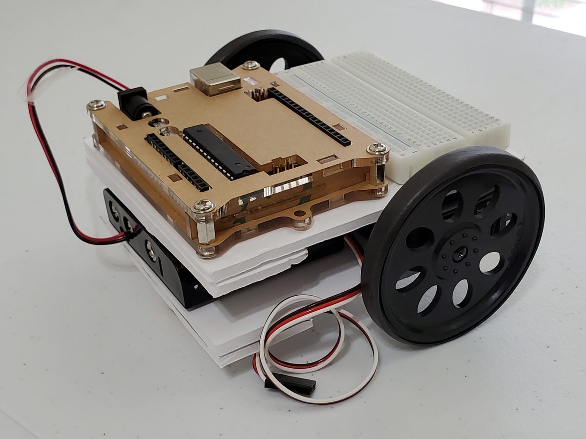
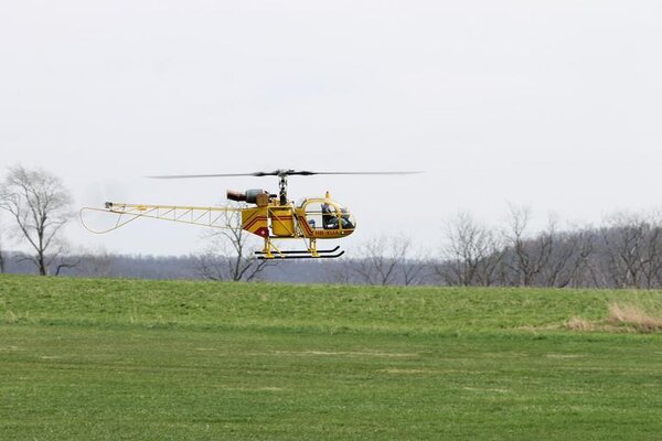
In this tutorial, we will learn how to derive the observation model for a two-wheeled mobile robot (I’ll explain what an observation model is below). Specifically, we’ll assume that our mobile robot is a differential drive robot like the one on the cover photo. A differential drive robot is one in which each wheel is driven independently from the other. 

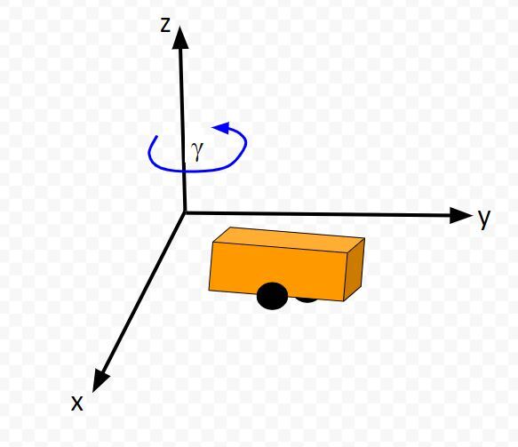
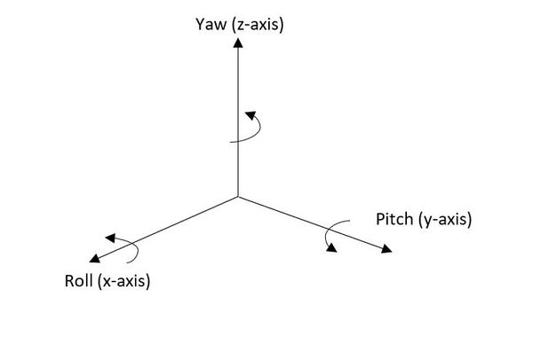
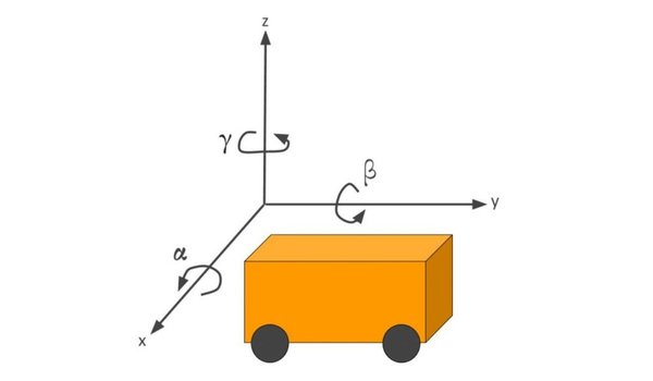
Below is a representation of a differential drive robot on a 3D coordinate plane with x, y, and z axes. The yaw angle γ represents the amount of rotation around the z axis as measured from the x axis. 

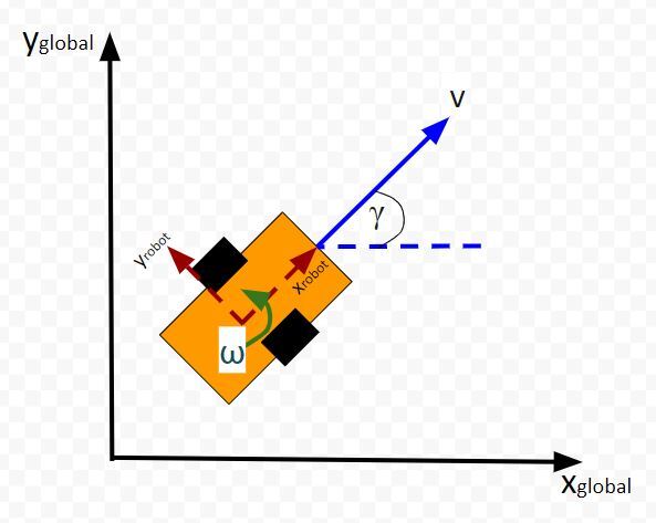
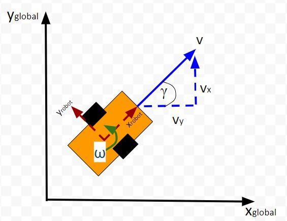
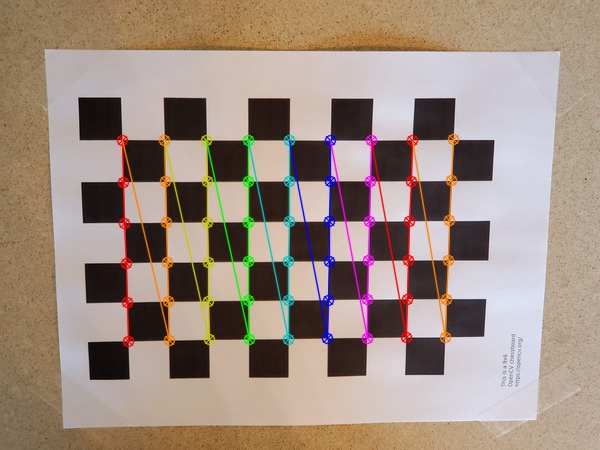
Here is the aerial view:

Real World Applications

• The most common application of deriving the observation model is when you want to do Kalman Filtering to smooth out noisy sensor measurements to generate a better estimate of the current state of a robotic system. I’ll cover this process in a future post. It is known as sensor fusion.

Prerequisites

• It is helpful if you have gone through my tutorial on state space modeling. Otherwise, if you understand the concept of state space modeling, jump right into this tutorial.

What is an Observation Model?

Typically, when a mobile robot is moving around in the world, we gather measurements from sensors to create an estimate of the state (i.e. where the robot is located in its environment and how it is oriented relative to some axis). 

An observation model does the opposite. Instead of converting sensor measurements to estimate the state, we use the state (or predicted state at the next timestep) to estimate (or predict) sensor measurements. The observation model is the mathematical equation that does this calculation.

You can understand why doing something like this is useful. Imagine you have a state space model of your mobile robot. You want the robot to move from a starting location to a goal location. In order to reach the goal location, the robot needs to know where it is located and which direction it is moving.

Suppose the robot’s sensors are really noisy, and you don’t trust its observations entirely to give you an accurate estimate of the current state. Or perhaps, all of a sudden, the sensor breaks, or generates erroneous data.

The observation model can help us in these scenarios. It enables you to predict what the sensor measurements would be at some timestep in the future. 

The observation model works by first using the state model to predict the state of the robot at that next timestep and then using that state prediction to infer what the sensor measurement would be at that point in time. 

You can then compute a weighted average (i.e. this is what you do during Kalman Filtering) of the predicted sensor measurements and the actual sensor observation at that timestep to create a better estimate of your state. 

This is what you do when you do Kalman Filtering. You combine noisy sensor observations with predicted sensor measurements (based on your state space model) to create a near-optimal estimate of the state of a mobile robot at some time t.

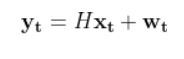
An observation model (also known as measurement model or sensor model) is a mathematical equation that represents a vector of predicted sensor measurements y at time t as a function of the state of a robotic system x at time t, plus some sensor noise (because sensors aren’t 100% perfect) at time t, denoted by vector w_t.

Here is the formal equation:

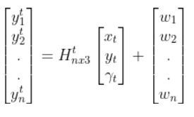
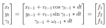
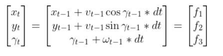
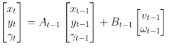
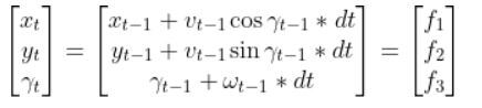
Because a mobile robot in 3D space has three states [x, y, yaw angle], in vector format, the observation model above becomes:

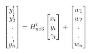
where:

• t = current time
• y vector (at left) = n predicted sensor observations at time t
• n = number of sensor observations (i.e. measurements) at time t 
• H = measurement matrix (used to convert the state at time t into predicted sensor observations at time t) that has n rows and 3 columns (i.e. a column for each state variable).
• w = the noise of each of the n sensor observations (you often get this sensor error information from the datasheet that comes when you purchase a sensor)

Sensor observations can be anything from distance to a landmark, to GPS readings, to ultrasonic distance sensor readings, to odometry readings….pretty much any number you can read from a robotic sensor that can help give you an estimate of the robot’s state (position and orientation) in the world.

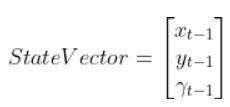
The reason why I say predicted measurements for the y vector is because they are not actual sensor measurements. Rather you are using the state of a mobile robot (i.e. the current location and orientation of a robot in 3D space) at time t-1 to predict the next state at time t, and then you use that next state (estimate) at time t to infer what the corresponding sensor measurement would be at that point in time t. 

How to Calculate the H Matrix

Let’s examine how to calculate H. The measurement matrix H is used to convert the predicted state estimate at time t into predicted sensor measurements at time t.

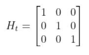
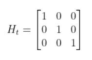
Imagine you had a sensor that could measure the x position, y position, and yaw angle (i.e. rotation angle around the z-axis) directly. What would H be? 

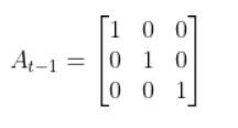
In this case, H will be the identity matrix since the estimated state maps directly to sensor measurements [x, y, yaw]. 

H has the same number of rows as sensor measurements and the same number of columns as states. Here is how the matrix would look in this scenario.

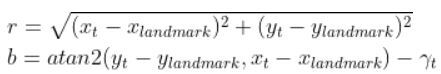
What if, for example, you had a landmark in your environment. How does the current state of the robot enable you to calculate the distance (i.e. range) to the landmark r and the bearing angle b to the landmark?

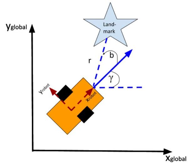
Using the Pythagorean Theorem and trigonometry, we get the following equations for the range r and bearing b:

Let’s put this in matrix form.

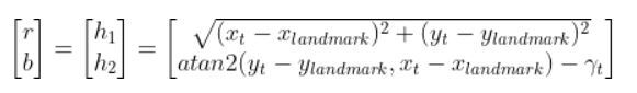
The formulas in the vector above are nonlinear (note the arctan2 function). They enable us to take the current state of the robot at time t and infer the corresponding sensor observations r and b at time t. 

Let’s linearize the model to create a linear observation model of the following form:

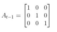
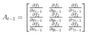
We have to calculate the Jacobian, just as we did when we calculated the A and B matrices in the state space modeling tutorial.

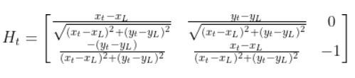
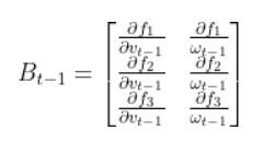
The formula for H_t is as follows:

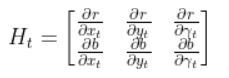
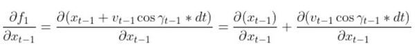
So we need to calculate 6 different partial derivatives. Here is what you should get:

Putting It All Together

The final observation model is as follows:

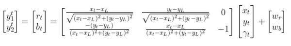
Equivalently, in some literature, you might see that all the stuff above is equal to:

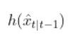
In fact, in the Wikipedia Extended Kalman Filter article, they replace time t with time k (not sure why because t is a lot more intuitive, but it is what it is).

Python Code Example for the Observation Model

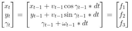
Let’s create an observation model in code. As a reminder, here is our robot model (as seen from above).

We’ll assume we have a sensor on our mobile robot that is able to give us exact measurements of the x_global position in meters, y_global position in meters, and yaw angle γ of the robot in radians at each timestep.

Therefore, as mentioned earlier, 

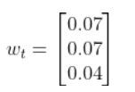
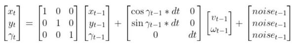
We’ll also assume that the corresponding noise (error) for our sensor readings is +/-0.07 m for the x position, +/-0.07 m for the y position, and +/-0.04 radians for the yaw angle. Therefore, here is the sensor noise vector:

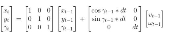
So, here is our equation:

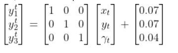
Suppose that the state of the robot at time t is [x=5.2, y=2.8, yaw angle=1.5708]. Because the yaw angle is 90 degrees (1.5708 radians), we know that the robot is heading due north relative to the global reference frame (i.e. the world or environment the robot is in).

What is the corresponding estimated sensor observation at time t given the current state of the robot at time t?

Here is the code:

import numpy as np

# Author: Addison Sears-Collins
# https://automaticaddison.com
# Description: An observation model for a differential drive mobile robot

# Measurement matrix H_t
# Used to convert the predicted state estimate at time t
# into predicted sensor measurements at time t.
# In this case, H will be the identity matrix since the 
# estimated state maps directly to state measurements from the 
# odometry data [x, y, yaw]
# H has the same number of rows as sensor measurements
# and same number of columns as states.
H_t = np.array([ 	[1.0,  0,   0],
					[  0,1.0,   0],
					[  0,  0, 1.0]])
				
# Sensor noise. This is a vector with the
# number of elements equal to the number of sensor measurements.
sensor_noise_w_t = np.array([0.07,0.07,0.04])
						
# The estimated state vector at time t in the global 
# reference frame
# [x_t, y_t, yaw_t]
# [meters, meters, radians]
state_estimate_t = np.array([5.2,2.8,1.5708])

def main():

	estimated_sensor_observation_y_t = H_t @ (
			state_estimate_t) + (
			sensor_noise_w_t)

	print(f'State at time t: {state_estimate_t}')
	print(f'Estimated sensor observations at time t: {estimated_sensor_observation_y_t}')

main()

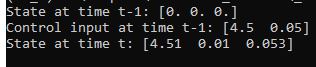
Here is the output:

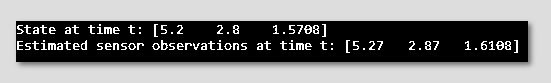
And that’s it folks. That linear observation model above enables you to convert the state at time t to estimated sensor observations at time t.

In a real robot application, we would use an Extended Kalman Filter to compute a weighted average of the estimated sensor reading using the observation model and the actual sensor reading that is mounted on your robot. In my next tutorial, I’ll show you how to implement an Extended Kalman Filter from scratch, building on the content we covered in this tutorial.

Keep building!

In this tutorial, we will learn how to create a state space model for a mobile robot. Specifically, we’ll take a look at a type of mobile robot called a differential drive robot. A differential drive robot is a robot like the one on the cover photo of this post, as well as this one below. It is called differential drive because each wheel is driven independently from the other. 

Prerequisites

• Basic linear algebra
  • You understand what a matrix and a vector are.
  • You know how to multiply two matrices together.
• You know what a partial derivative is.
• Optional: Python 3.7 or higher (just needed for the last part of this tutorial)

There are a lot of tutorials on YouTube if you don’t have the prerequisites above (e.g. Khan Academy).

What is a State Space Model?

A state space model (often called the state transition model) is a mathematical equation that represents the motion of a robotic system from one timestep to the next. It shows how the current position (e.g. X, Y coordinate) and orientation (yaw (heading) angle γ) of the robot in the world is impacted by changes to the control inputs into the robot (e.g. velocity in meters per second…often represented by the variable v).

Note: In a real-world scenario, we would need to represent the world the robot is in (e.g. a room in your house, etc.) as an x,y,z coordinate grid.

Deriving the Equations

Consider the mobile robot below. It is moving around on the flat x-y coordinate plane.

Let’s look at it from an aerial view.

What is the position and orientation of the robot in the world (i.e. global reference frame)? The position and orientation of a robot make up what we call the state vector.

Note that x and y as well as the yaw angle γ are in the global reference frame.

The yaw angle γ describes the rotation around the z-axis (coming out of the page in the image above) in the counterclockwise direction (from the x axis). The units for the yaw angle are typically radians.

ω is the rotation rate (i.e. angular velocity or yaw rate) around the global z axis. Typically the units on this variable is radians per second.

The velocity of the robot v is in terms of the robot reference frame (labeled x_robot and y_robot). 

In terms of the global reference frame we can break v down into two components: 

• velocity in the x direction v_x 
• velocity in the y direction v_y. 

In most of my applications, I express the velocity in meters per second.

Using trigonometry, we know that:

• cos(γ) = v_x/v 
• sin(γ) = v_x/v 

Therefore, with respect to the global reference frame, the robot’s motion equations are as follows:

linear velocity in the x direction = v_x = vcos(γ)

linear velocity in the y direction = v_y = vsin(γ)

angular velocity around the z axis = ω

Now let’s suppose at time t-1, the robot has the current state (x position, y position, yaw angle γ):

We move forward one timestep dt. What is the state of the robot at time t? In other words, where is the robot location, and how is the robot oriented? 

Remember that distance = velocity * time. 

Therefore,

Converting the Equations to a State Space Model

We now know how to describe the motion of the robot mathematically. However the equation above is nonlinear. For some applications, like using the Kalman Filter (I’ll cover Kalman Filters in a future post), we need to make our state space equations linear.

How do we take this equation that is nonlinear (note the cosines and sines)…

…and convert it into a form that looks like the equation of a line? In mathematical jargon, we want to make the equation above a linear discrete-time state space model of the following form.

where:

x_t is our entire current state vector [x_t, y_t,γ_t]  (i.e. note x_t in bold is the entire state vector…don’t get that confused with x_t, which is just the x coordinate of the robot at time t)

x_t-1 is the state of the mobile robot at the previous timestep: [x_t-1, y_t-1,γ_t-1]

u_t-1 represents the control input vector at the previous timestep [v_t-1, ω_t-1] = [forward velocity, angular velocity]. 

I’ll get to what the A and B matrices represent later in this post.

Let’s write out the full form of the linear state space model equation:

Let’s go through this equation term by term to make sure we understand everything so we can convert this equation below into the form above:

How to Calculate the A Matrix

A is a matrix. The number of rows in the A matrix is equal to the number of states, and the number of columns in the A matrix is equal to the number of states. In this mobile robot example, we have three states.

The A matrix expresses how the state of the system [x position,y position,yaw angle γ] changes from t-1 to t when no control command is executed (i.e. when we don’t give any speed (velocity) commands to the robot). 

Typically a robot on wheels only drives when the wheels are commanded to turn. Therefore, for this case, A is the identity matrix (Note that A is sometimes F in the literature).

In other applications, A might not be the identity matrix. An example is a helicopter. The state of a helicopter flying around in the air changes even if you give it no velocity command. Gravity will pull the helicopter downward to Earth regardless of what you do. It will eventually crash if you give it no velocity commands.

Formally, to calculate A, you start with the equation for each state vector variable. In our mobile robot example, that is this stuff below.

Our system is expressed as a nonlinear system now because the state is a function of cosines and sines (which are nonlinear trigonometric operations).

To get our state space model in this form…

…we need to “linearize” the nonlinear equations. To do this, we need to calculate the Jacobian, which is nothing more than a fancy name for “matrix of partial derivatives.” 

Do you remember the equation for a straight line from grade school: y=mx+b? m is the slope. It is “change in y / change in x”.

The Jacobian is nothing more than a multivariable form of the slope m. It is “change in y1/x1, change in y2/x2, change in y3/x3, etc….”  

You can consider the Jacobian a slope on steroids. It represents how fast a group of variables (as opposed to just one variable…(e.g. m = rise/run = change in y/change in x) are changing with respect to another group of variables.

You start with this here:

You then calculate the partial derivative of the state vector at time t with respect to the states at time t-1. Don’t be scared at all the funny symbols inside this matrix A. When you’re calculating the Jacobian matrix, you calculate each partial derivative, one at a time.

You will have to calculate 9 partial derivatives in total for this example. 

Again, if you are a bit rusty on calculating partial derivatives, there are some good tutorials online. We’ll do an example calculation now so you can see how this works.

Let’s calculate the first partial derivative in the upper left corner of the matrix.

and

So, 1 goes in the upper-left corner of the matrix.

If you calculate all 9 partial derivatives above, you’ll get:

which is the identity matrix.

If you actually calculate these partial derivatives, you will get the following for A_{t-1}:

Since we assume 0 for the control inputs, A becomes the identity matrix.

The assumption that the control inputs (v_{t-1} and ω_{t-1}) are zero when calculating the A matrix is based on the physical characteristics of the differential drive mobile robot and the purpose of the A matrix in the state space model.

Physical characteristics of the robot:

A differential drive mobile robot typically only moves when its wheels are commanded to turn. If no control input is given (i.e., the robot is not commanded to move), the robot will remain stationary, and its position and orientation will not change from one time step to the next.

Purpose of the A matrix:

In the state space model, the A matrix is used to express how the state of the system [x position, y position, yaw angle γ] changes from time step t-1 to t when no control command is executed. It represents the natural evolution of the system state without any external influence from the control inputs.

By setting v_{t-1} and ω_{t-1} to zero when calculating the A matrix, we are essentially modeling the behavior of the robot when it is not being actively controlled. This is a valid assumption because we are interested in understanding how the system state evolves on its own, without any control commands.

Linearization at a Specific Point

• Linearizing a nonlinear system involves finding the Jacobian matrix at a specific operating point.
• The chosen operating point here is where the robot is stationary (i.e., no control inputs).

Use Case: Kalman Filtering

The assumption that the A matrix is an identity matrix when no control inputs are given is particularly useful in the context of Kalman filtering for a few reasons:

1. Simplification of the prediction step: In the Kalman filter, the prediction step is responsible for estimating the robot’s state at the next time step based on its current state and the control inputs. By assuming that the A matrix is an identity matrix, the prediction step becomes simpler. The predicted state is essentially the same as the current state if no control inputs are given, which aligns with the physical behavior of the robot.
2. Focus on the effect of control inputs: With the A matrix being an identity matrix, the Kalman filter can focus more on the effect of the control inputs on the robot’s state. The B matrix captures how the control inputs (linear and angular velocities) influence the change in the robot’s position and orientation. This allows the Kalman filter to effectively incorporate the control inputs into the state estimation process. We’ll calculate the B matrix in the next section.
3. Modeling the uncertainty: The Kalman filter is designed to handle uncertainty in the robot’s motion and measurements. By assuming that the A matrix is an identity matrix, the uncertainty in the robot’s motion is primarily attributed to the control inputs and the process noise. The process noise can be modeled to account for factors like wheel slippage, uneven surfaces, or other disturbances that affect the robot’s motion. The Kalman filter uses this uncertainty information to estimate the robot’s state more accurately.
4. Computational efficiency: Using an identity matrix for the A matrix can lead to more efficient computations in the Kalman filter. Since the identity matrix has a simple structure (1s on the diagonal and 0s elsewhere), it can simplify the matrix calculations involved in the prediction and update steps of the filter. This can be beneficial when running the Kalman filter on resource-constrained systems or when real-time performance is critical.

It’s important to note that the assumption of an identity matrix for A is specific to the case when no control inputs are given. In the overall Kalman filter algorithm, the actual control inputs (linear and angular velocities) are still used in the prediction step to estimate the robot’s state at the next time step.

By leveraging this assumption, the Kalman filter can more effectively estimate the robot’s state, account for uncertainty, and incorporate the effect of control inputs, all while maintaining computational efficiency. This makes it a powerful tool for state estimation and localization in mobile robot applications.

How to Calculate the B Matrix

The B matrix in our running example of a mobile robot is a 3×2 matrix. 

The B matrix has the same number of rows as the number of states and has the same number of columns as the number of control inputs. 

The control inputs in this example are the linear velocity (v) and the angular velocity around the z axis, ω (also known as the “yaw rate”).

The B matrix expresses how the state of the system (i.e. [x,y,γ]) changes from t-1 to t due to the control commands (i.e. control inputs v and ω)

Since we’re dealing with a robotic car here, we know that if we apply forward and angular velocity commands to the car, the car will move.

The equation for B is as follows. We need to calculate yet another Jacobian matrix. However, unlike our calculation for the A matrix, we need to compute the partial derivative of the state vector at time t with respect to the control inputs at time t-1.

Remember the equations for f₁, f₂, and f₃:

If you calculate the 6 partial derivatives, you’ll get this for the B matrix below:

Putting It All Together

Ok, so how do we get from this:

Into this form:

We now know the A and B matrices, so we can plug those in. The final state space model for our differential drive robot is as follows:

where v_t-1 is the linear velocity of the robot in the robot’s reference frame, and ω_t-1 is the angular velocity in the robot’s reference frame.

And there you have it. If you know the current position of the robot (x,y), the orientation of the robot (yaw angle γ), the linear velocity of the robot, the angular velocity of the robot, and the change in time from one timestep to the next, you can calculate the state of the robot at the next timestep.

Adding Process Noise

The world isn’t perfect. Sometimes the robot might not act the way you would expect when you want it to execute a specific velocity command. 

It is often common to add a noise term to the state space model to account for randomness in the world. The equation would then be:

Python Code Example for the State Space Model

In this section, I’ll show you code in Python for the state space model we have developed in this tutorial. We will assume:

• The robot begins at the origin at a yaw angle of 0 radians. 
• We then apply a forward velocity of 4.5 meters per second at time t-1 and an angular velocity of 0.05 radians per second.

The output will show the state of the robot at the next timestep, time t. I’ll name the file state_space_model.py.

Make sure you have NumPy installed before you run the code. NumPy is a scientific computing library for Python.

If you’re using Anaconda, you can type:

conda install numpy

Alternatively, you can type:

pip install numpy

Here is the code. You can copy and paste this code into your favorite IDE and then run it.

import numpy as np

# Author: Addison Sears-Collins
# https://automaticaddison.com
# Description: A state space model for a differential drive mobile robot

# A matrix
# 3x3 matrix -> number of states x number of states matrix
# Expresses how the state of the system [x,y,yaw] changes 
# from t-1 to t when no control command is executed.
# Typically a robot on wheels only drives when the wheels are commanded
# to turn.
# For this case, A is the identity matrix.
# A is sometimes F in the literature.
A_t_minus_1 = np.array([[1.0,  0,   0],
                        [  0,1.0,   0],
                        [  0,  0, 1.0]])
						
# The estimated state vector at time t-1 in the global 
# reference frame
# [x_t_minus_1, y_t_minus_1, yaw_t_minus_1]
# [meters, meters, radians]
state_estimate_t_minus_1 = np.array([0.0,0.0,0.0])

# The control input vector at time t-1 in the global 
# reference frame
# [v, yaw_rate]
# [meters/second, radians/second]
# In the literature, this is commonly u.
control_vector_t_minus_1 = np.array([4.5, 0.05])

# Noise applied to the forward kinematics (calculation
# of the estimated state at time t from the state
# transition model of the mobile robot). This is a vector
# with the number of elements equal to the number of states
process_noise_v_t_minus_1 = np.array([0.01,0.01,0.003])

yaw_angle = 0.0 # radians
delta_t = 1.0 # seconds

def getB(yaw,dt):
  """
  Calculates and returns the B matrix
  3x2 matix -> number of states x number of control inputs
  The control inputs are the forward speed and the
  rotation rate around the z axis from the x-axis in the 
  counterclockwise direction.
  [v, yaw_rate]
  Expresses how the state of the system [x,y,yaw] changes
  from t-1 to t due to the control commands (i.e. control
  input).
  :param yaw: The yaw (rotation angle around the z axis) in rad 
  :param dt: The change in time from time step t-1 to t in sec
	"""
  B = np.array([[np.cos(yaw)*dt, 0],
                [np.sin(yaw)*dt, 0],
                [0, dt]])
  return B

def main():
  state_estimate_t = A_t_minus_1 @ (
    state_estimate_t_minus_1) + (
    getB(yaw_angle, delta_t)) @ (
    control_vector_t_minus_1) + (
    process_noise_v_t_minus_1)

  print(f'State at time t-1: {state_estimate_t_minus_1}')
  print(f'Control input at time t-1: {control_vector_t_minus_1}')
  print(f'State at time t: {state_estimate_t}') # State after delta_t seconds

main()

Run the code:

python state_space_model.py

Here is the output:

And that’s it for the fundamentals of state space modeling. Once you know the physics of how a robotic system moves from one timestep to the next, you can create a mathematical model in state space form. 

Keep building!