Make sure the network name and password are inside quotes.
Save the file.
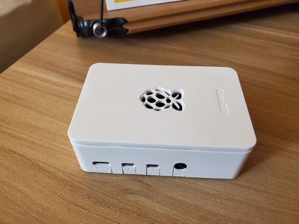
Set Up the Raspberry Pi
Safely remove the microSD Card Reader from your laptop.
Remove the microSD card from the card reader.
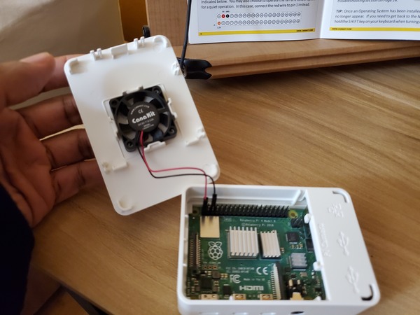
Insert the microSD card into the bottom of the Raspberry Pi.
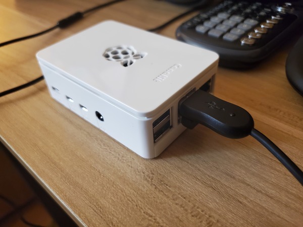
Connect a keyboard and a mouse to the USB 3.0 ports of the Raspberry Pi.
Connect an HDMI monitor to the Raspberry Pi using the Micro HDMI cable connected to the Main MIcro HDMI port (which is labeled HDMI 0).
Connect the 3A USB-C Power Supply to the Raspberry Pi. You should see the computer boot.
Log in using “ubuntu” as both the password and login ID. You will have to do this multiple times.
You will then be asked to change your password.
Type:
sudo reboot
Type the command:
hostname -I
You will see the IP address of your Raspberry Pi. Mine is 192.168.254.68. Write this number down on a piece of paper because you will need it later.
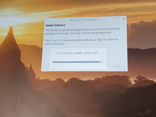
Now update and upgrade the packages.
sudo apt update
sudo apt upgrade
Now, install a desktop.
sudo apt install xubuntu-desktop
Installing the desktop should take around 20-30 minutes or so.
Once that is done, it will ask you what you want as your default display manager. I’m going to use gdm3.
Wait for that to download.
Reboot your computer.
sudo reboot
Your desktop should show up.
Type in your password and press ENTER.
Click on Activities in the upper left corner of the screen to find applications.
If you want to see a Windows-like desktop, type the following commands:
cd ~/.cache/sessions/
Remove any files in there.
Type:
rm
Then press the Tab key and press Enter.
Now type:
xfdesktop
Connect to Raspberry Pi from Your Personal Computer
Follow the steps for Putty under step 9b at this link to connect to your Raspberry Pi from your personal computer.
Install Raspbian
Now, we will install the Raspbian operating system. Turn off the Raspberry Pi, and remove the microSD card.
Insert the default microSD card that came with the kit.
Turn on the Raspberry Pi.
You should see an option to select “Raspbian Full [RECOMMENDED]”. Click the checkbox beside that.
Change the language to your desired language.
Click Wifi networks, and type in the password of your network.
Click Install.
Click Yes to confirm.
Wait while the operating system installs.
You’ll get a message that the operating system installed successfully.
Now follow all the steps from Step 7 of this tutorial. All the software updates at the initial startup take a really long time, so be patient. You can even go and grab lunch and return. It might not look like the progress bar is moving, but it is.
In this tutorial, we will learn the fundamentals of imitation learning by playing a video game. We will teach an agent how to play Flappy Bird, one of the most popular video games in the world way back in 2014.
The objective of the game is to get a bird to move through a sequence of pipes without touching them. If the bird touches them, he falls out of the sky.
Ubuntu Linux (If you’re on Windows or MacOS, you can download a virtual machine and install Ubuntu. Don’t be scared if you’ve never used Ubuntu Linux before. It is a great operating system, and you’ll get comfortable with it in no time.)
In order to understand what imitation learning is, it is first helpful to understand what reinforcement learning is all about.
Reinforcement learning is a machine learning method that involves training a software “agent” (i.e. algorithm) to learn through trial and error. The agent is rewarded by the environment when it does something good and punished when it does something bad. “Good” and “bad” behavior in this case are defined beforehand by the programmer.
The idea behind reinforcement learning is that the agent learns over time the best actions it must take in different situations (i.e. states of the environment) in order to maximize its rewards and minimize its punishment. That stuff in bold in the previous sentence is formally known as the agent’s optimal policy.
One of the problems with reinforcement learning is that it takes a long time for an agent to learn through trial and error. Knowing the optimal action to take in any given state of the environment means that the agent has to explore a lot of different random actions in different states of the environment in order to fully learn.
You can imagine how infeasible this gets as the environment gets more complex. Imagine a robot learning how to make a breakfast of bacon and eggs. Assume the robot is in your kitchen and has no clue what bacon and eggs are. It has no clue how to use a stove. It has no clue how to use a spatula. It doesn’t even know how to use a frying pan.
The only thing the robot has is the feedback it receives when it takes an action that is in accordance with the goal of getting it to make bacon and eggs.
You could imagine that it could take decades for a robot to learn how to cook bacon and eggs this way, through trial and error. As humans, we don’t have that much time, so we need to use some other machine learning method that is more efficient.
And this brings us to imitation learning. Imitation learning helps address the shortcomings of reinforcement learning. It is also known as learning from demonstrations.
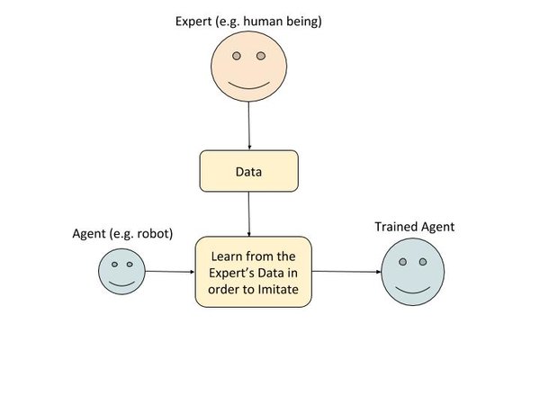
In imitation learning, during the training phase, the agent first observes the actions of an expert (e.g. a human). The agent keeps a record of what actions the expert took in different states of the environment. The agent uses this data to create a policy that attempts to mimic the expert.
Diagram of How Imitation Learning Works
Babies and little kids learn this way. They imitate the actions of their parents. For example, I remember learning how to make my bed by watching my mom and then trying to imitate what she did.
Now, at runtime, the environment won’t be exactly similar as it was when the agent was in the training phase observing the expert. The agent will try to approximate the best action to take in any given state based on what it learned while watching the expert during the training phase.
Imitation learning is a powerful technique that works well when:
The number of states of the environment is large (e.g. in a kitchen, where you can have near infinite ways a kitchen can be arranged)
The rewards are sparse (e.g. there are only a few actions a robot can take that will bring him closer to the goal of making a bacon and egg breakfast)
An expert is available.
Going back to our bacon and eggs example, a robotic agent doing imitation learning would observe a human making bacon and eggs from scratch. The robot would then try to imitate that process.
In the case of reinforcement learning, the robotic agent will take random actions and will receive a reward every time it takes an action that is consistent with the goal of cooking bacon and eggs.
For example, if the robot cracks an egg into a frying pan, it would receive a reward. If the robot cracks an egg on the floor, it would not receive a reward.
After a considerable amount of time (maybe years!), the robot would finally be smart enough (based on performance metrics established by the programmer) to know how to cook bacon and eggs.
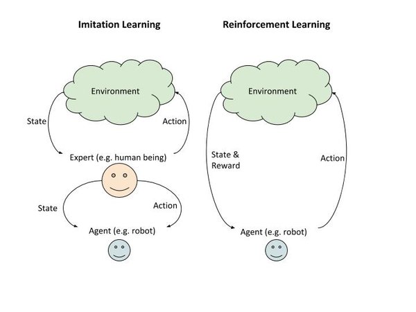
So you see that the runtime behavior of imitation learning and reinforcement learning are the same. The difference is in how the agent learns during the training phase.
In reinforcement learning, the agent learns through trial and error by receiving varying rewards from the environment in response to its action.
In imitation learning, the agent learns by watching an expert. It observes the action the expert took in various states.
Because there is no explicit reward in the case of imitation learning, the agent only becomes as good as the teacher (but never better). Thus, if you have a bad expert, you will have a bad agent.
The agent doesn’t know the reward (consequences) of taking a specific action in a certain state. The graphic below further illustrates the difference between reinforcement learning and imitation learning.
So with that background, let’s dive into implementing an imitation learning algorithm to teach an agent to play Flappy Bird.
You can find the instructions for installing FlappyBird at this link, but let’s run through the process as it can be a bit tricky. Go slow, so you make sure you get all the necessary libraries.
Open up a terminal window.
Install all the dependencies for Python 3.X listed here. I’ll copy and paste all that below, but if you have any issues, check out the link. You can copy and paste the command below into your terminal.
You don’t have to know what each library does, but in case you’re interested, you can take a look at the Ubuntu packages page to get a complete description.
We’re not done yet with all the installations. Let’s install the PyGame Learning Environment (PLE) now by copying the entire repository to our computer. It already includes Flappy Bird.
Let’s write a Python script in order to use the game environment.
Open a new terminal window.
Go to the PyGame-Learning-Environment directory.
cd PyGame-Learning-Environment
We will create the script flappybird1.py. Open the text editor to create a new file.
gedit flappybird1.py
Here is the full code. You can find a full explanation of the methods at the PyGameLearning Environment website. The function getScreenRGB retrieves the state of the environment in the form of red/green/blue image pixels:
# Import Flappy Bird from games library in
# Python Learning Environment (PLE)
from ple.games.flappybird import FlappyBird

# Import PyGame Learning Environment
from ple import PLE

# Create a game instance
game = FlappyBird()

# Pass the game instance to the PLE
p = PLE(game, fps=30, display_screen=True, force_fps=False)

# Initialize the environment
p.init()


actions = p.getActionSet()
print(actions) # 119 to flap wings, or None to do nothing
action_dict = {0: actions[1], 1:actions[0]}

reward = 0.0

for i in range(10000):
  if p.game_over():
    p.reset_game()

  state = p.getScreenRGB()
  action = 1
  reward = p.act(action_dict[action])
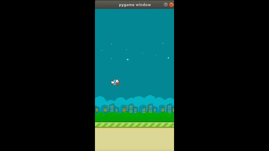
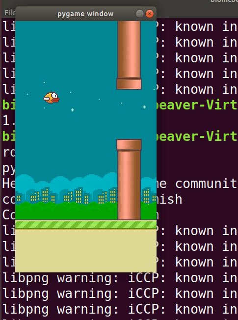
Now, run the program using the following command:
python3 flappybird1.py
Here is what you should see:
Here is flappybird2.py. The agent takes a random action at each iteration of the game.
# Import Flappy Bird from games library in
# Python Learning Environment (PLE)
from ple.games.flappybird import FlappyBird

# Import PyGame Learning Environment
from ple import PLE

# Import Numpy
import numpy as np

class NaiveAgent():
  """
  This is a naive agent that just picks actions at random.
  """
  def __init__(self,actions):
    self.actions = actions

  def pickAction(self, reward, obs):
    return self.actions[np.random.randint(0, len(self.actions))]

# Create a game instance
game = FlappyBird()

# Pass the game instance to the PLE
p = PLE(game)

# Create the agent
agent = NaiveAgent(p.getActionSet())

# Initialize the environment
p.init()

actions = p.getActionSet()
action_dict = {0: actions[1], 1:actions[0]}

reward = 0.0

for f in range(15000):

  # If the game is over
  if p.game_over():
    p.reset_game()

  action = agent.pickAction(reward, p.getScreenRGB())
  reward = p.act(action)

  if f > 1000:
    p.display_screen = True
    p.force_fps = False # Slow screen
Implement the Dataset Aggregation Algorithm (DAgger)
How the DAgger Algorithm Works
In this section, we will implement the Dataset Aggregation Algorithm (DAgger) and apply it to FlappyBird.
The DAgger algorithm is a type of imitation learning algorithm that is intended to help address the problem of the agent “memorizing” the actions of the expert in different states. It is time-consuming to watch the expert do every combination of possible states of the environment, so we need the expert to give the agent some guidance on what to do in the event the agent makes errors.
In the first phase, we first let the expert take action in the environment and keep track of what action the expert took in a variety of states of the environment. This phase creates an initial “policy”, a collection of state-expert action pairs.
Then for the second phase, we add a twist to the situation. The expert continues to act, and we record the expert’s actions. However, the environment doesn’t change according to the expert’s actions. Rather it changes in response to the policy from phase 1. The environment is “ignoring” the actions of the expert.
In the meantime, a new policy is created that maps the state to the expert’s actions.
You might now wonder, which policy would the agent choose? The policy from phase 1 or phase 2. One method is to pick one at random. Another method (and the one often preferred in practice) is to hold out a subset of states of the environment and test which one performs the best.
We now need to install TensorFlow, the popular machine learning library.
Open a new terminal window, and type the following command (wait a bit as it will take some time to download).
pip3 install tensorflow
Run FlappyBird
Now we need to run FlappyBird with the imitation learning algorithm. Since the game has no real expert, we have to have our algorithm load a special file (included in the GitHub folder that we will clone in a second) that has the expert’s pre-prepared policy.
Eventually, you should see the results of each game spit out, with the bird’s score on the far right. Notice that the agent’s score gets above 100 after only a few minutes of training.
That’s it for imitation learning. If you want to learn more, I highly suggest you check out Andrea Lonza’s book, Reinforcement Learning Algorithms with Python, that does a great job teaching imitation learning.
Neural networks are the workhorses of the rapidly growing field known as deep learning. Neural networks are used for all sorts of applications where a prediction of some sort is desired. Here are some examples:
Predicting the type of objects in an image or video
Sales forecasting
Speech recognition
Medical diagnosis
Risk management
and countless other applications…
In this post, I will explain how neural networks make those predictions by boiling these structures down to their fundamental parts and then building up from there.
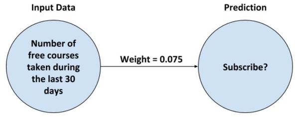
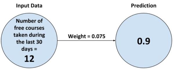
Imagine you run a business that provides short online courses for working professionals. Some of your courses are free, but your best courses require the students to pay for a subscription.
You want to create a neural network to predict if a free student is likely to upgrade to a paid subscription. Let’s create the most basic neural network you can make.
OK, so there is our neural network. To implement this neural network on a computer, we need to translate this diagram into a software program. Let’s do that now using Python, the most popular language for machine learning.
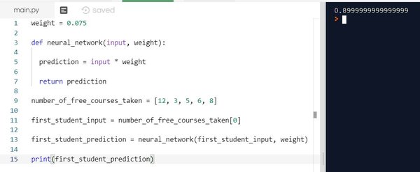
# Declare a variable named weight and
# initiate it with a value
weight = 0.075

# Create a method called neural_network that
# takes as inputs, the input data (number of
free courses a student has taken during the
# last 30 days) and the weight of the connection.
# The method returns the prediction.

def neural_network(input, weight):

  # The input data multiplied by the weight
  # equals the prediction
  prediction = input * weight

  # This is the output
  return prediction
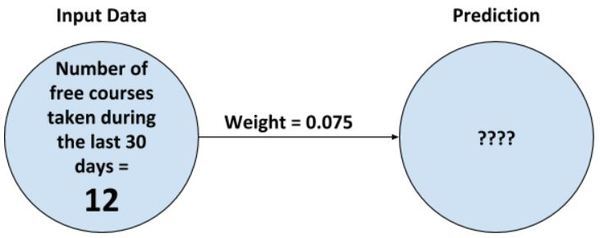
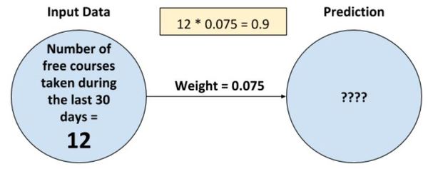
So we currently have five students, all of whom are free students. The number of free courses these users have taken during the last 30 days is 12, 3, 5, 6, and 8. Let’s code this in Python as a list.
number_of_free_courses_taken = [12, 3, 5, 6, 8]
Let’s make a prediction for the first student, the one who has taken 12 free courses over the last 30 days.
Now let’s put the diagram into code.
# Extract the first value of the list...12...
# and store into a variable named input
first_student_input = number_of_free_courses_taken[0]

# Call the neural_network method and store the
# prediction result into a variable
first_student_prediction = neural_network(
                         first_student_input, weight)

# Print the prediction
print(first_student_prediction)
OK. We have finished the code. Let’s see how it looks all together.
Open a Jupyter Notebook and run the code above, or run the code inside your favorite Python IDE.
Here is what I got:
What did you get? Did you get 0.9? If so, congratulations!
Let’s see what is happening when we run our code. We called the neural_network method. The first operation performed inside that method is to multiply the input by the weight and return the result. In this case, the input is 12, and the weight is 0.075. The result is 0.9.
0.9 is stored in the first_student_prediction variable.
And this, my friend, is the most basic building block of a neural network. A neural network in its simplest form consists of one or more weights which you can multiply by input data to make a prediction.
Let’s take a look at some questions you might have at this stage.
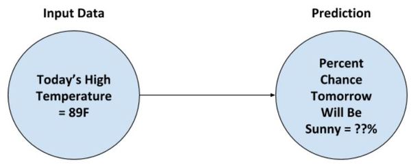
What kind of input data can go into a neural network?
Real numbers that can be measured or calculated somewhere in the real world. Yesterday’s high temperature, a medical patient’s blood pressure reading, previous year’s rainfall, or average annual rainfall are all valid inputs into a neural network. Negative numbers are totally acceptable as well.
A good rule of thumb is, if you can quantify it, you can use it as an input into a neural network. It is best to use input data into a neural network that you think will be relevant for making the prediction you desire.
For example, if you are trying to create a neural network to predict if a patient has breast cancer or not, how many fingers a person has probably not going to be all that relevant. However, how many days per month a patient exercises is likely to be a relevant piece of input data that you would want to feed into your neural network.
What does a neural network predict?
A neural network outputs some real number. In some neural network implementations, we can do some fancy mathematics to limit the output to some real number between 0 and 1. Why would we want to do that? Well in some applications we might want to output probabilities. Let me explain.
Suppose you want to predict the probability that tomorrow will be sunny. The input into a neural network to make such a prediction could be today’s high temperature.
If the output is some number like 0.30, we can interpret this as a 30% change of the weather being sunny tomorrow given today’s high temperature. Pretty cool huh!
We don’t have to limit the output to between 0 and 1. For example, let’s say we have a neural network designed to predict the price of a house given the house’s area in square feet. Such a network might tell us, “given the house’s area in square feet, the predicted price of the house is $432,000.”
What happens if the neural network’s predictions are incorrect?
The neural network will adjust its weights so that the next time it makes a more accurate prediction. Recall that the weights are multiplied by the input values to make a prediction.
What is a neural network really learning?
A neural network is learning the best possible set of weights. “Best” in the context of neural networks means the weights that minimize the prediction error.
Remember, the core math operation in a neural network is multiplication, where the simplest neural network is:
Input Value * Weight = Prediction
How does the neural network find the best set of weights?
Short answer: Trial and error
Long answer: A neural network starts out with random numbers for weights. It then takes in a single input data point, makes a prediction, and then sees if its prediction was either too high or too low. The neural network then adjusts its weight(s) accordingly so that the next time it sees the same input data point, it makes a more accurate prediction.
Once the weights are adjusted, the neural network is fed the next data point, and so on. A neural network gets better and better each time it makes a prediction. It “learns” from its mistakes one data point at a time.
Do you notice something here?
Standard neural networks have no memory. They are fed an input data point, make a prediction, see how close the prediction was to reality, adjust the weights accordingly, and then move on to the next data point. At each step of the learning process of a neural network, it has no memory of the most recent prediction it made.
Standard neural networks focus on one input data point at a time. For example, in our subscriber prediction neural network we built earlier in this tutorial, if we feed our neural network number_of_free_courses_taken[1], it will have no clue what it predicted when number_of_free_courses_taken[0] was the input value.