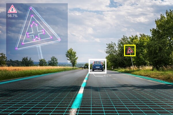
In this tutorial, we will build an application to detect and classify traffic signs. By the end of this tutorial, you will be able to build this:
Our goal is to build an early prototype of a system that can be used in a self-driving car or other type of autonomous vehicle.
Real-World Applications
- Self-driving cars/autonomous vehicles
Prerequisites
- Python 3.7 or higher
- You have TensorFlow 2 Installed. I’m using Tensorflow 2.3.1.
- Windows 10 Users, see this post.
- If you want to use GPU support for your TensorFlow installation, you will need to follow these steps. If you have trouble following those steps, you can follow these steps (note that the steps change quite frequently, but the overall process remains relatively the same).
- This post can also help you get your system setup, including your virtual environment in Anaconda (if you decide to go this route).
Helpful Tip
When you work through tutorials in robotics or any other field in technology, focus on the end goal. Focus on the authentic, real-world problem you’re trying to solve, not the tools that are used to solve the problem.
Don’t get bogged down in trying to understand every last detail of the math and the libraries you need to use to develop an application.
Don’t get stuck in rabbit holes. Don’t try to learn everything at once.
You’re trying to build products not publish research papers. Focus on the inputs, the outputs, and what the algorithm is supposed to do at a high level. As you’ll see in this tutorial, you don’t need to learn all of computer vision before developing a robust road sign classification system.
Get a working road sign detector and classifier up and running; and, at some later date when you want to add more complexity to your project or write a research paper, then feel free to go back to the rabbit holes to get a thorough understanding of what is going on under the hood.
Trying to understand every last detail is like trying to build your own database from scratch in order to start a website or taking a course on internal combustion engines to learn how to drive a car.
Let’s get started!
Find a Data Set
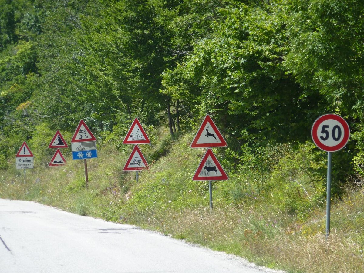
The first thing we need to do is find a data set of road signs.
We will use the popular German Traffic Sign Recognition Benchmark data set. This data set consists of more than 43 different road sign types and 50,000+ images. Each image contains a single traffic sign.
Download the Data Set
Go to this link, and download the data set. You will see three data files.
- Training data set
- Validation data set
- Test data set
The data files are .p (pickle) files.
What is a pickle file? Pickling is where you convert a Python object (dictionary, list, etc.) into a stream of characters. That stream of characters is saved as a .p file. This process is known as serialization.
Then, when you want to use the Python object in another script, you can use the Pickle library to convert that stream of characters back to the original Python object. This process is known as deserialization.
Training, validation, and test data sets in computer vision can be large, so pickling them in order to save them to your computer reduces storage space.
Installation and Setup
We need to make sure we have all the software packages installed.
Make sure you have NumPy installed, a scientific computing library for Python.
If you’re using Anaconda, you can type:
conda install numpy
Alternatively, you can type:
pip install numpy
Install Matplotlib, a plotting library for Python.
For Anaconda users:
conda install -c conda-forge matplotlib
Otherwise, you can install like this:
pip install matplotlib
Install scikit-learn, the machine learning library:
conda install -c conda-forge scikit-learn
Write the Code
Open a new Python file called load_road_sign_data.py
Here is the full code for the road sign detection and classification system:
# Project: How to Detect and Classify Road Signs Using TensorFlow
# Author: Addison Sears-Collins
# Date created: February 13, 2021
# Description: This program loads the German Traffic Sign
# Recognition Benchmark data set
import warnings # Control warning messages that pop up
warnings.filterwarnings("ignore") # Ignore all warnings
import matplotlib.pyplot as plt # Plotting library
import matplotlib.image as mpimg
import numpy as np # Scientific computing library
import pandas as pd # Library for data analysis
import pickle # Converts an object into a character stream (i.e. serialization)
import random # Pseudo-random number generator library
from sklearn.model_selection import train_test_split # Split data into subsets
from sklearn.utils import shuffle # Machine learning library
from subprocess import check_output # Enables you to run a subprocess
import tensorflow as tf # Machine learning library
from tensorflow import keras # Deep learning library
from tensorflow.keras import layers # Handles layers in the neural network
from tensorflow.keras.models import load_model # Loads a trained neural network
from tensorflow.keras.utils import plot_model # Get neural network architecture
# Open the training, validation, and test data sets
with open("./road-sign-data/train.p", mode='rb') as training_data:
train = pickle.load(training_data)
with open("./road-sign-data/valid.p", mode='rb') as validation_data:
valid = pickle.load(validation_data)
with open("./road-sign-data/test.p", mode='rb') as testing_data:
test = pickle.load(testing_data)
# Store the features and the labels
X_train, y_train = train['features'], train['labels']
X_valid, y_valid = valid['features'], valid['labels']
X_test, y_test = test['features'], test['labels']
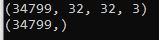
# Output the dimensions of the training data set
# Feel free to uncomment these lines below
#print(X_train.shape)
#print(y_train.shape)
# Display an image from the data set
i = 500
#plt.imshow(X_train[i])
#plt.show() # Uncomment this line to display the image
#print(y_train[i])
# Shuffle the image data set
X_train, y_train = shuffle(X_train, y_train)
# Convert the RGB image data set into grayscale
X_train_grscale = np.sum(X_train/3, axis=3, keepdims=True)
X_test_grscale = np.sum(X_test/3, axis=3, keepdims=True)
X_valid_grscale = np.sum(X_valid/3, axis=3, keepdims=True)
# Normalize the data set
# Note that grayscale has a range from 0 to 255 with 0 being black and
# 255 being white
X_train_grscale_norm = (X_train_grscale - 128)/128
X_test_grscale_norm = (X_test_grscale - 128)/128
X_valid_grscale_norm = (X_valid_grscale - 128)/128
# Display the shape of the grayscale training data
#print(X_train_grscale.shape)
# Display a sample image from the grayscale data set
i = 500
# squeeze function removes axes of length 1
# (e.g. arrays like [[[1,2,3]]] become [1,2,3])
#plt.imshow(X_train_grscale[i].squeeze(), cmap='gray')
#plt.figure()
#plt.imshow(X_train[i])
#plt.show()
# Get the shape of the image
# IMG_SIZE, IMG_SIZE, IMG_CHANNELS
img_shape = X_train_grscale[i].shape
#print(img_shape)
# Build the convolutional neural network's (i.e. model) architecture
cnn_model = tf.keras.Sequential() # Plain stack of layers
cnn_model.add(tf.keras.layers.Conv2D(filters=32,kernel_size=(3,3),
strides=(3,3), input_shape = img_shape, activation='relu'))
cnn_model.add(tf.keras.layers.Conv2D(filters=64,kernel_size=(3,3),
activation='relu'))
cnn_model.add(tf.keras.layers.MaxPooling2D(pool_size = (2, 2)))
cnn_model.add(tf.keras.layers.Dropout(0.25))
cnn_model.add(tf.keras.layers.Flatten())
cnn_model.add(tf.keras.layers.Dense(128, activation='relu'))
cnn_model.add(tf.keras.layers.Dropout(0.5))
cnn_model.add(tf.keras.layers.Dense(43, activation = 'sigmoid')) # 43 classes
# Compile the model
cnn_model.compile(loss='sparse_categorical_crossentropy', optimizer=(
keras.optimizers.Adam(
0.001, beta_1=0.9, beta_2=0.999, epsilon=1e-07, amsgrad=False)), metrics =[
'accuracy'])
# Train the model
history = cnn_model.fit(x=X_train_grscale_norm,
y=y_train,
batch_size=32,
epochs=50,
verbose=1,
validation_data = (X_valid_grscale_norm,y_valid))
# Show the loss value and metrics for the model on the test data set
score = cnn_model.evaluate(X_test_grscale_norm, y_test,verbose=0)
print('Test Accuracy : {:.4f}'.format(score[1]))
# Plot the accuracy statistics of the model on the training and valiation data
accuracy = history.history['accuracy']
val_accuracy = history.history['val_accuracy']
epochs = range(len(accuracy))
## Uncomment these lines below to show accuracy statistics
# line_1 = plt.plot(epochs, accuracy, 'bo', label='Training Accuracy')
# line_2 = plt.plot(epochs, val_accuracy, 'b', label='Validation Accuracy')
# plt.title('Accuracy on Training and Validation Data Sets')
# plt.setp(line_1, linewidth=2.0, marker = '+', markersize=10.0)
# plt.setp(line_2, linewidth=2.0, marker= '4', markersize=10.0)
# plt.xlabel('Epochs')
# plt.ylabel('Accuracy')
# plt.grid(True)
# plt.legend()
# plt.show() # Uncomment this line to display the plot
# Save the model
cnn_model.save("./road_sign.h5")
# Reload the model
model = load_model('./road_sign.h5')
# Get the predictions for the test data set
predicted_classes = np.argmax(cnn_model.predict(X_test_grscale_norm), axis=-1)
# Retrieve the indices that we will plot
y_true = y_test
# Plot some of the predictions on the test data set
for i in range(15):
plt.subplot(5,3,i+1)
plt.imshow(X_test_grscale_norm[i].squeeze(),
cmap='gray', interpolation='none')
plt.title("Predict {}, Actual {}".format(predicted_classes[i],
y_true[i]), fontsize=10)
plt.tight_layout()
plt.savefig('road_sign_output.png')
plt.show()
How the Code Works
Let’s go through each snippet of code in the previous section so that we understand what is going on.
Load the Image Data
The first thing we need to do is to load the image data from the pickle files.
with open("./road-sign-data/train.p", mode='rb') as training_data:
  train = pickle.load(training_data)
with open("./road-sign-data/valid.p", mode='rb') as validation_data:
  valid = pickle.load(validation_data)
with open("./road-sign-data/test.p", mode='rb') as testing_data:
  test = pickle.load(testing_data)
Create the Train, Test, and Validation Data Sets
We then split the data set into a training set, testing set and validation set.
X_train, y_train = train['features'], train['labels']
X_valid, y_valid = valid['features'], valid['labels']
X_test, y_test = test['features'], test['labels']
print(X_train.shape)
print(y_train.shape)
i = 500
plt.imshow(X_train[i])
plt.show() # Uncomment this line to display the image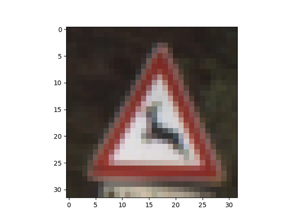
Shuffle the Training Data
Shuffle the data set to make sure that we don’t have unwanted biases and patterns.
X_train, y_train = shuffle(X_train, y_train)Convert Data Sets from RGB Color Format to Grayscale
Our images are in RGB format. We convert the images to grayscale so that the neural network can process them more easily.
X_train_grscale = np.sum(X_train/3, axis=3, keepdims=True)
X_test_grscale  = np.sum(X_test/3, axis=3, keepdims=True)
X_valid_grscale  = np.sum(X_valid/3, axis=3, keepdims=True)

i = 500
plt.imshow(X_train_grscale[i].squeeze(), cmap='gray')
plt.figure()
plt.imshow(X_train[i])
plt.show()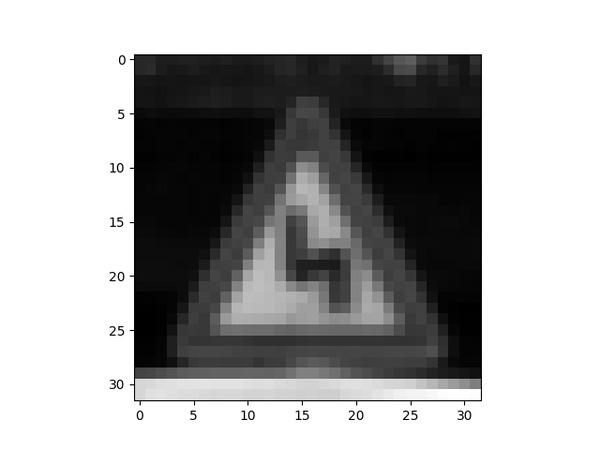
Normalize the Data Sets to Speed Up Training of the Neural Network
We normalize the images to speed up training and improve the neural network’s performance.
X_train_grscale_norm = (X_train_grscale - 128)/128
X_test_grscale_norm = (X_test_grscale - 128)/128
X_valid_grscale_norm = (X_valid_grscale - 128)/128
Build the Convolutional Neural Network
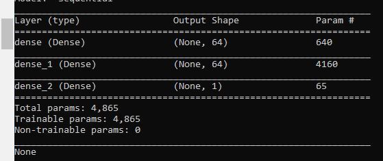
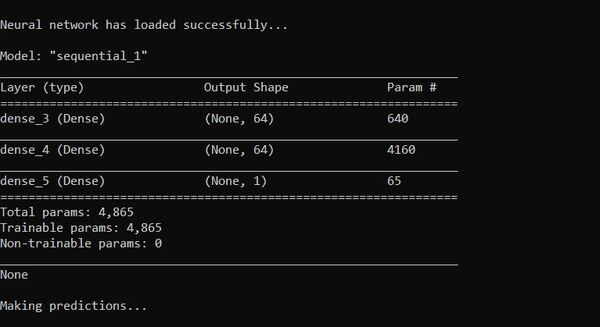
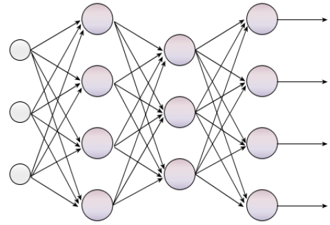
In this snippet of code, we build the neural network’s architecture.
cnn_model = tf.keras.Sequential() # Plain stack of layers
cnn_model.add(tf.keras.layers.Conv2D(filters=32,kernel_size=(3,3),
  strides=(3,3), input_shape = img_shape, activation='relu'))
cnn_model.add(tf.keras.layers.Conv2D(filters=64,kernel_size=(3,3),
  activation='relu'))
cnn_model.add(tf.keras.layers.MaxPooling2D(pool_size = (2, 2)))
cnn_model.add(tf.keras.layers.Dropout(0.25))
cnn_model.add(tf.keras.layers.Flatten())
cnn_model.add(tf.keras.layers.Dense(128, activation='relu'))
cnn_model.add(tf.keras.layers.Dropout(0.5))
cnn_model.add(tf.keras.layers.Dense(43, activation = 'sigmoid')) # 43 classes
Compile the Convolutional Neural Network
The compilation process sets the model’s architecture and configures its parameters.
cnn_model.compile(loss='sparse_categorical_crossentropy', optimizer=(
  keras.optimizers.Adam(
  0.001, beta_1=0.9, beta_2=0.999, epsilon=1e-07, amsgrad=False)), metrics =[
  'accuracy'])
Train the Convolutional Neural Network
We now train the neural network on the training data set.
history = cnn_model.fit(x=X_train_grscale_norm,
  y=y_train,
  batch_size=32,
  epochs=50,
  verbose=1,
  validation_data = (X_valid_grscale_norm,y_valid))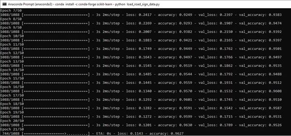
Display Accuracy Statistics
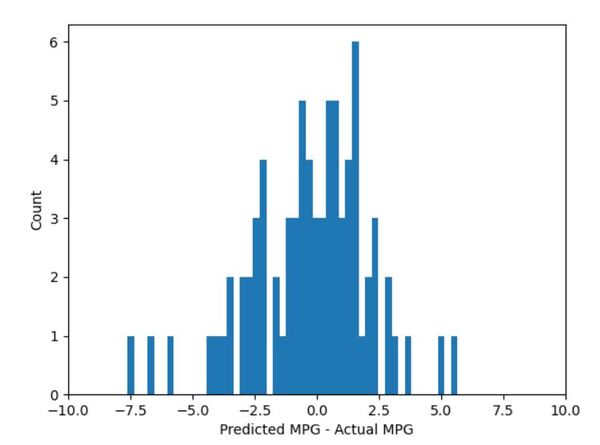
We then take a look at how well the neural network performed. The accuracy on the test data set was ~95%. Pretty good!
score = cnn_model.evaluate(X_test_grscale_norm, y_test,verbose=0)
print('Test Accuracy : {:.4f}'.format(score[1]))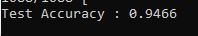
accuracy = history.history['accuracy']
val_accuracy = history.history['val_accuracy']
epochs = range(len(accuracy))

line_1 = plt.plot(epochs, accuracy, 'bo', label='Training Accuracy')
line_2 = plt.plot(epochs, val_accuracy, 'b', label='Validation Accuracy')
plt.title('Accuracy on Training and Validation Data Sets')
plt.setp(line_1, linewidth=2.0, marker = '+', markersize=10.0)
plt.setp(line_2, linewidth=2.0, marker= '4', markersize=10.0)
plt.xlabel('Epochs')
plt.ylabel('Accuracy')
plt.grid(True)
plt.legend()
plt.show() # Uncomment this line to display the plot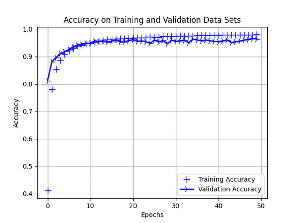
Save the Convolutional Neural Network to a File
We save the trained neural network so that we can use it in another application at a later date.
cnn_model.save("./road_sign.h5")Verify the Output
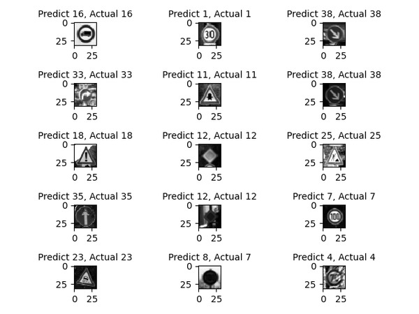
Finally, we take a look at some of the output to see how our neural network performs on unseen data. You can see in this subset that the neural network correctly classified 14 out of the 15 test examples.
# Reload the model
model = load_model('./road_sign.h5')

# Get the predictions for the test data set
predicted_classes = np.argmax(cnn_model.predict(X_test_grscale_norm), axis=-1)

# Retrieve the indices that we will plot
y_true = y_test

# Plot some of the predictions on the test data set
for i in range(15):
  plt.subplot(5,3,i+1)
  plt.imshow(X_test_grscale_norm[i].squeeze(),
    cmap='gray', interpolation='none')
  plt.title("Predict {}, Actual {}".format(predicted_classes[i],
    y_true[i]), fontsize=10)
plt.tight_layout()
plt.savefig('road_sign_output.png')
plt.show()
That’s it. Keep building!