Why Most Machine Learning Books Suck

Good teaching is work. Great teaching is a lot of work. Mediocre teaching is no work at all.
Addison Sears-Collins (2019)

Yes, the title is provocative, but somebody had to say it. Here is a quick list why most machine learning books are a waste of time. I’ll get into each point later in this post.

Subscript and Superscript Soup
Too Much Focus on Irrelevant Minutiae
Teaching to the Tools Instead of the Problem
No Common Language
Author Has No Training on How to Teach
Using Words Like “Basically”, “Simple”, and “Easy”
Show Me Don’t Tell Me
Here is What Well Written Textbooks Look Like

Most of the “introductory” machine learning books (textbooks, especially) suck. While the subject matter in these books is supposed to be introductory, the way in which concepts are explained is not introductory at all. Simple concepts are often explained with such complex jargon and mathematical symbol soup that the underlying ideas get totally lost.

If you want to see mental masturbation at its finest, just pick up any of the popular machine learning textbooks used in machine learning courses at colleges and universities around the world.

So many of these machine learning textbooks spend pages and pages explaining machine learning without actually doing machine learning with step-by-step fully worked real-world examples (I presume because the publisher wants to limit the page count). It is kind of like learning how to play tennis by having someone explain to you how to play tennis vs. getting out there on the court and actually playing!

While reading these books, I always find myself asking these questions:

Why write an introductory book if the explanations are so convoluted that only an expert can understand?
Why ask end-of-chapter questions and provide no answer key?
Why provide no step-by-step practice with real-world examples?

Feedback and deliberate practice is a critical part of building confidence as you learn a new skill. Most of the “introduction” to machine learning books lose sight of this concept. Authors need to realize that you need to start with teeny tiny baby steps when you are writing for beginners.

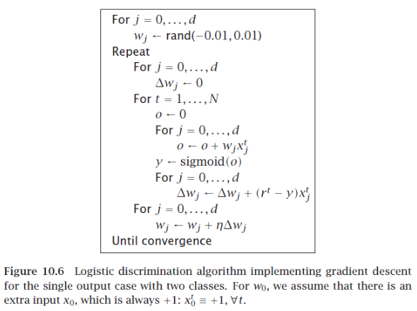
Subscript and Superscript Soup

Take a look at this excerpt from a popular Introduction to Machine Learning textbook where the author attempts to explain logistic regression.

subscript-soup — Source: *Introduction to Machine Learning*

Wtf?

This example hits on one of my biggest annoyances about machine learning books. The algorithms and mathematical equations contain so many variables, subscripts, and superscripts that you need to make a glossary on a separate sheet of paper just to keep track of it all because it would be utterly impossible to retain everything in your head while trying to decipher the points the author is trying to make. This kind of practice gets in the way of learning as well as your ability to see the big picture.

Most of these “introduction” to machine learning books are written for people who already have a deep expertise in the subject. The subscript and superscript soup present in these books are as understandable to me as Ancient Greek.

Too Much Focus on Irrelevant Minutiae

Take a look at this page taken from another popular Machine Learning book where the author introduces the K-Means clustering algorithm.

What the heck is this guy talking about? I had to double check the preface to see if this book was written for beginners or experts (i.e. it was written for beginners). To the average undergrad who wants to go out and get a job applying machine learning to real-world problems, how important is it to know all these mathematical details upfront?

Answer: Not very important. Rarely will you ever need to know these details, and if you do, just look them up. Most textbooks focus way too much on the minutiae (as if they are writing an academic research paper) and not enough on how to apply this knowledge to solve real-world problems.

At no point do these authors convey:

Why does knowing this matter?
What value does knowing this have on a real-world application as well as my ability to get and retain a job in this field. Most beginners don’t want to go on to get PhDs and do research. Some do, but most of the readers do not.

Teaching to the Tools Instead of the Problem

Machine learning textbooks need to teach to the problem, not to the tools and the underlying mathematics. They need to first tell you why something is important. The easiest way to do this is to explain a concept by starting with a real-world problem.

Most textbooks, instead, do it the other way around. They teach you the intricate details of the tool in isolation, teach you some proof, and then (in rare cases), apply the concept to a problem (a problem which almost never resembles the types of problems you would face in the real world at a job).

Authors need to show readers how machine learning fits into the big picture (i.e. the other tools a beginner might already be familiar with, like statistics or data analysis). At the end of the day, machine learning is just a tool. It is not a panacea.

It is just a tool, just like the World Wide Web is a tool…just like a programming language like Python is a tool…or just like Microsoft Excel is a tool.

Machine Learning is to an engineer what a wrench is to a mechanic. A mechanic does not need to know how to build a wrench in order to use it. He just needs to know how to use it to solve a problem. The vast majority of people will not need to know the underlying proofs and mathematics at such a detailed level in order to succeed in the workplace (unless you become a researcher, in that case, you will be trying to build a better wrench).

tool_wall_tool_storage_0 — Machine Learning is a tool in the toolbox

Machine learning textbooks need to start with a real-world problem, then work through that problem, set-by-step, and explain the mathematics on an as-needed basis, not just throw it on the page for the sake of pretending to be mathematically rigorous.

If you decide to deep dive into research later on in your career, THEN pick up the mathematics on an as-needed basis.

I don’t need to know how an internal combustion engine is built to be an awesome driver, and most companies will hire you based on your problem-solving ability, not on your ability to write proofs of off-the-shelf algorithms…so problem solving is what books need to focus on.

No Common Language

It does not help that there is no common language in machine learning. There are sometimes a dozen different ways to say the same thing (feature, attribute, predictor, x-variables, independent variables, etc.) or (target, class, response variable, y-variable, hypothesis). These multiple ways of saying the same thing make it totally confusing for a beginner, and rarely do authors point out the fact that there are a myriad of ways of saying the same thing.

Author Has No Training on How to Teach

Many of these authors are accustomed to writing for an expert audience (via academic research papers) and have not properly developed the skill of breaking down complex subject matter into easy-to-understand, digestible bite-sized pieces that would be understandable by a competent beginner.

Elementary and high school teachers must get a degree or diploma in teaching. They have to endure hundreds of hours of instruction on how to teach and how to deal with different learning styles. Most machine learning textbook authors have not had this training.

I find that the best teachers of a subject are often students who are one step removed from having learned the subject. It is fresh in their minds, and they still remember what it is like to be a beginner.

Using Words Like “Basically”, “Simple”, and “Easy”

A favorite of machine learning textbook authors it to make the assumption that the reader already understands a “simple” concept that’s necessary to understand the new topic. This is frustrating for someone new.

So many of these textbooks use terms like “simple,” “straightforward,” “easy,” “obvious,” and “basically,” which hurts a beginner’s confidence if he is not easily able to grasp the material. This is a huge pet peeve of mine. Words like these have no place in a book claiming to be an “introduction.”

You’re trying to climb the machine learning mountain. The author is already at the top of the mountain. The author forgot how hard the struggle was to get to the top. The author forgot what it is like to even take the first step because it has been so long. It all seems easy after you’ve been there, done that.

It would be like Michael Jordan teaching someone how to play basketball. Some things are so intuitive and second nature to him that, although he is the best basketball player that ever lived, he might not be the best one to teach it because he is so far removed from what it was like as a beginner, learning the basics, when even the smallest steps are difficult and not second nature.

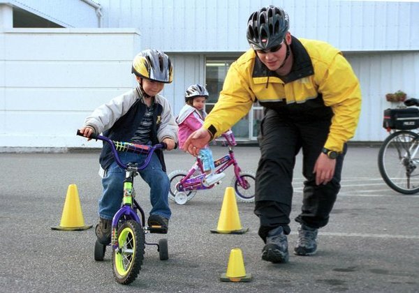
Similarly, you might know how to ride a bicycle really well. However, try to teach someone else how to ride a bicycle. You will notice that teaching someone how to ride a bike is different from being a really good bike rider. In order to teach someone how to ride a bike, you have to take what you know and break it down into teeny tiny parts. The ability to do this well is a skill in and of itself…one that takes time and practice to get good at.

When you learn something, and especially if it is something you’ve spent decades immersed in, it’s intuition to you. Most machine learning books are especially bad about this. They just assume that you understand exactly what is going on. They do not explain. It was just “if this, then that.” They speak in generalities and hand-wavy language when the beginner needs step-by-step detail. They use machine learning and math to explain machine learning and math.

They do not realize that in order to teach someone something, it is best to tie the new concept to a concept that the beginner might already be familiar with.

Again, the best teachers in my experience are those that are one step removed from learning a subject as they have the knowledge fresh in their mind and remember clearly what it is like to be a beginner.

Show Me Don’t Tell Me

Authors need to stop introducing a new concept by explaining it. Instead, they need to use the following teaching aids:

Analogies: Connect the current knowledge to previous knowledge that most beginners would have.
Pictures and Diagrams: Draw a picture to help me visualize the concept.
Real-world Examples: Why does this concept matter? Show me a real-world example of this concept in practice, solving an actual problem. Tell me a story.
Layman’s Terms: Explain a term in basic plain language. Act as if you are explaining a concept to a five-year-old child.

Here is What Well Written Textbooks Look Like

Here is what a well written textbooks for beginners should look like. Consider these textbooks among the GOATs (i.e. greatest of all time) of textbooks:

The books above are an absolute joy to learn from. They will make you rethink the way introductory textbooks should be written.

For you “Introduction” to machine learning authors out there, take note.

Real-World Applications

Any computer vision application written in Python that handles images or videos could use NumPy.

Let’s get started!

Prerequisites

Python 3.7 or higher

Installation and Setup

We now need to make sure we have all the software packages installed. Check to see if you have OpenCV installed on your machine. If you are using Anaconda, you can type:

conda install -c conda-forge opencv

Alternatively, you can type:

pip install opencv-python

Make sure you have NumPy installed, a scientific computing library for Python.

If you’re using Anaconda, you can type:

conda install numpy

Alternatively, you can type:

pip install numpy

Write the Code

Open up a new Python file called numpy_array_creation.py.

Here is the full code:

# Project: How To Create a NumPy Array
# Author: Addison Sears-Collins
# Date created: February 24, 2021
# Description: Basics of using the NumPy library

import numpy as np # Import the NumPy library

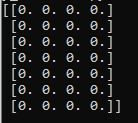
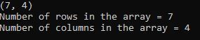
# Create and print a two dimensional array with 7 rows and 4 columns
my_array = np.zeros((7,4))
#print(my_array)

# Print the data type
#print(my_array.dtype)

# Print the dimensions of the array
#print(my_array.shape)
#print("Number of rows in the array = {}".format(my_array.shape[0]))
#print("Number of columns in the array = {}".format(my_array.shape[1]))
	
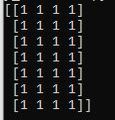
# Create an array of ones that contains 8-bit unsigned integers
my_array_ones = np.ones((7,4), dtype=np.uint8)
#print(my_array_ones)

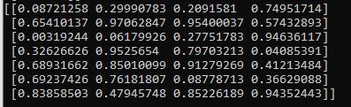
# Create an array of random numbers
my_array_random_nums = np.random.rand(7,4)
#print(my_array_random_nums)

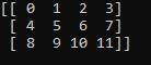
# Create a 4x3 two-dimensional array (i.e. a matrix)
my_2d_array = np.array([[0, 1, 2, 3],
                        [4, 5, 6, 7],
                        [8, 9, 10, 11]])
												
#print(my_2d_array)

# Extract the value from the matrix on row 3, column 2 (i.e. the 9)
#print(my_2d_array[2,1])

Code Output

# Create and print a two dimensional array with 7 rows and 4 columns
my_array = np.zeros((7,4))
print(my_array)

# Print the data type
print(my_array.dtype)

# Print the dimensions of the array
print(my_array.shape)
print("Number of rows in the array = {}".format(my_array.shape[0]))
print("Number of columns in the array = {}".format(my_array.shape[1]))

# Create an array of ones that contains 8-bit unsigned integers
my_array_ones = np.ones((7,4), dtype=np.uint8)
print(my_array_ones)

# Create an array of random numbers
my_array_random_nums = np.random.rand(7,4)
print(my_array_random_nums)

# Create a 4x3 two-dimensional array (i.e. a matrix)
my_2d_array = np.array([[0, 1, 2, 3],
                        [4, 5, 6, 7],
                        [8, 9, 10, 11]])												
print(my_2d_array)

# Extract the value from the matrix on row 3, column 2 (i.e. the 9)
print(my_2d_array[2,1])

That’s it. Keep building!

How to Detect and Classify Road Signs Using TensorFlow

In this tutorial, we will build an application to detect and classify traffic signs. By the end of this tutorial, you will be able to build this:

Our goal is to build an early prototype of a system that can be used in a self-driving car or other type of autonomous vehicle.

Real-World Applications

Self-driving cars/autonomous vehicles

Prerequisites

Python 3.7 or higher
You have TensorFlow 2 Installed. I’m using Tensorflow 2.3.1.
- Windows 10 Users, see this post.
- If you want to use GPU support for your TensorFlow installation, you will need to follow these steps. If you have trouble following those steps, you can follow these steps (note that the steps change quite frequently, but the overall process remains relatively the same).
- This post can also help you get your system setup, including your virtual environment in Anaconda (if you decide to go this route).

Helpful Tip

When you work through tutorials in robotics or any other field in technology, focus on the end goal. Focus on the authentic, real-world problem you’re trying to solve, not the tools that are used to solve the problem.

Don’t get bogged down in trying to understand every last detail of the math and the libraries you need to use to develop an application.

Don’t get stuck in rabbit holes. Don’t try to learn everything at once.

You’re trying to build products not publish research papers. Focus on the inputs, the outputs, and what the algorithm is supposed to do at a high level. As you’ll see in this tutorial, you don’t need to learn all of computer vision before developing a robust road sign classification system.

Get a working road sign detector and classifier up and running; and, at some later date when you want to add more complexity to your project or write a research paper, then feel free to go back to the rabbit holes to get a thorough understanding of what is going on under the hood.

Trying to understand every last detail is like trying to build your own database from scratch in order to start a website or taking a course on internal combustion engines to learn how to drive a car.

Let’s get started!

Find a Data Set

The first thing we need to do is find a data set of road signs.

We will use the popular German Traffic Sign Recognition Benchmark data set. This data set consists of more than 43 different road sign types and 50,000+ images. Each image contains a single traffic sign.

Download the Data Set

Go to this link, and download the data set. You will see three data files.

Training data set
Validation data set
Test data set

The data files are .p (pickle) files.

What is a pickle file? Pickling is where you convert a Python object (dictionary, list, etc.) into a stream of characters. That stream of characters is saved as a .p file. This process is known as serialization.

Then, when you want to use the Python object in another script, you can use the Pickle library to convert that stream of characters back to the original Python object. This process is known as deserialization.

Training, validation, and test data sets in computer vision can be large, so pickling them in order to save them to your computer reduces storage space.

Installation and Setup

We need to make sure we have all the software packages installed.

Make sure you have NumPy installed, a scientific computing library for Python.

If you’re using Anaconda, you can type:

conda install numpy

Alternatively, you can type:

pip install numpy

Install Matplotlib, a plotting library for Python.

For Anaconda users:

conda install -c conda-forge matplotlib

Otherwise, you can install like this:

pip install matplotlib

Install scikit-learn, the machine learning library:

conda install -c conda-forge scikit-learn

Write the Code

Open a new Python file called load_road_sign_data.py

Here is the full code for the road sign detection and classification system:

# Project: How to Detect and Classify Road Signs Using TensorFlow
# Author: Addison Sears-Collins
# Date created: February 13, 2021
# Description: This program loads the German Traffic Sign 
#              Recognition Benchmark data set

import warnings # Control warning messages that pop up
warnings.filterwarnings("ignore") # Ignore all warnings

import matplotlib.pyplot as plt # Plotting library
import matplotlib.image as mpimg
import numpy as np # Scientific computing library 
import pandas as pd # Library for data analysis
import pickle # Converts an object into a character stream (i.e. serialization)
import random # Pseudo-random number generator library
from sklearn.model_selection import train_test_split # Split data into subsets
from sklearn.utils import shuffle # Machine learning library
from subprocess import check_output # Enables you to run a subprocess
import tensorflow as tf # Machine learning library
from tensorflow import keras # Deep learning library
from tensorflow.keras import layers # Handles layers in the neural network
from tensorflow.keras.models import load_model # Loads a trained neural network
from tensorflow.keras.utils import plot_model # Get neural network architecture

# Open the training, validation, and test data sets
with open("./road-sign-data/train.p", mode='rb') as training_data:
  train = pickle.load(training_data)
with open("./road-sign-data/valid.p", mode='rb') as validation_data:
  valid = pickle.load(validation_data)
with open("./road-sign-data/test.p", mode='rb') as testing_data:
  test = pickle.load(testing_data)

# Store the features and the labels
X_train, y_train = train['features'], train['labels']
X_valid, y_valid = valid['features'], valid['labels']
X_test, y_test = test['features'], test['labels']

# Output the dimensions of the training data set
# Feel free to uncomment these lines below
#print(X_train.shape)
#print(y_train.shape)

# Display an image from the data set
i = 500
#plt.imshow(X_train[i])
#plt.show() # Uncomment this line to display the image
#print(y_train[i])

# Shuffle the image data set
X_train, y_train = shuffle(X_train, y_train)

# Convert the RGB image data set into grayscale
X_train_grscale = np.sum(X_train/3, axis=3, keepdims=True)
X_test_grscale  = np.sum(X_test/3, axis=3, keepdims=True)
X_valid_grscale  = np.sum(X_valid/3, axis=3, keepdims=True)

# Normalize the data set
# Note that grayscale has a range from 0 to 255 with 0 being black and
# 255 being white
X_train_grscale_norm = (X_train_grscale - 128)/128 
X_test_grscale_norm = (X_test_grscale - 128)/128
X_valid_grscale_norm = (X_valid_grscale - 128)/128

# Display the shape of the grayscale training data
#print(X_train_grscale.shape)

# Display a sample image from the grayscale data set
i = 500
# squeeze function removes axes of length 1 
# (e.g. arrays like [[[1,2,3]]] become [1,2,3]) 
#plt.imshow(X_train_grscale[i].squeeze(), cmap='gray') 
#plt.figure()
#plt.imshow(X_train[i])
#plt.show()

# Get the shape of the image
# IMG_SIZE, IMG_SIZE, IMG_CHANNELS
img_shape = X_train_grscale[i].shape
#print(img_shape)

# Build the convolutional neural network's (i.e. model) architecture
cnn_model = tf.keras.Sequential() # Plain stack of layers
cnn_model.add(tf.keras.layers.Conv2D(filters=32,kernel_size=(3,3), 
  strides=(3,3), input_shape = img_shape, activation='relu'))
cnn_model.add(tf.keras.layers.Conv2D(filters=64,kernel_size=(3,3), 
  activation='relu'))
cnn_model.add(tf.keras.layers.MaxPooling2D(pool_size = (2, 2)))
cnn_model.add(tf.keras.layers.Dropout(0.25))
cnn_model.add(tf.keras.layers.Flatten())
cnn_model.add(tf.keras.layers.Dense(128, activation='relu'))
cnn_model.add(tf.keras.layers.Dropout(0.5))
cnn_model.add(tf.keras.layers.Dense(43, activation = 'sigmoid')) # 43 classes

# Compile the model
cnn_model.compile(loss='sparse_categorical_crossentropy', optimizer=(
  keras.optimizers.Adam(
  0.001, beta_1=0.9, beta_2=0.999, epsilon=1e-07, amsgrad=False)), metrics =[
  'accuracy'])
	
# Train the model
history = cnn_model.fit(x=X_train_grscale_norm,
  y=y_train,
  batch_size=32,
  epochs=50,
  verbose=1,
  validation_data = (X_valid_grscale_norm,y_valid))
	
# Show the loss value and metrics for the model on the test data set
score = cnn_model.evaluate(X_test_grscale_norm, y_test,verbose=0)
print('Test Accuracy : {:.4f}'.format(score[1]))

# Plot the accuracy statistics of the model on the training and valiation data
accuracy = history.history['accuracy']
val_accuracy = history.history['val_accuracy']
epochs = range(len(accuracy))
## Uncomment these lines below to show accuracy statistics
# line_1 = plt.plot(epochs, accuracy, 'bo', label='Training Accuracy')
# line_2 = plt.plot(epochs, val_accuracy, 'b', label='Validation Accuracy')
# plt.title('Accuracy on Training and Validation Data Sets')
# plt.setp(line_1, linewidth=2.0, marker = '+', markersize=10.0)
# plt.setp(line_2, linewidth=2.0, marker= '4', markersize=10.0)
# plt.xlabel('Epochs')
# plt.ylabel('Accuracy')
# plt.grid(True)
# plt.legend()
# plt.show() # Uncomment this line to display the plot

# Save the model
cnn_model.save("./road_sign.h5")

# Reload the model
model = load_model('./road_sign.h5')

# Get the predictions for the test data set
predicted_classes = np.argmax(cnn_model.predict(X_test_grscale_norm), axis=-1)

# Retrieve the indices that we will plot
y_true = y_test

# Plot some of the predictions on the test data set
for i in range(15):
  plt.subplot(5,3,i+1)
  plt.imshow(X_test_grscale_norm[i].squeeze(), 
    cmap='gray', interpolation='none')
  plt.title("Predict {}, Actual {}".format(predicted_classes[i], 
    y_true[i]), fontsize=10)
plt.tight_layout()
plt.savefig('road_sign_output.png')
plt.show()

How the Code Works

Let’s go through each snippet of code in the previous section so that we understand what is going on.

Load the Image Data

The first thing we need to do is to load the image data from the pickle files.

with open("./road-sign-data/train.p", mode='rb') as training_data:
  train = pickle.load(training_data)
with open("./road-sign-data/valid.p", mode='rb') as validation_data:
  valid = pickle.load(validation_data)
with open("./road-sign-data/test.p", mode='rb') as testing_data:
  test = pickle.load(testing_data)

Create the Train, Test, and Validation Data Sets

We then split the data set into a training set, testing set and validation set.

X_train, y_train = train['features'], train['labels']
X_valid, y_valid = valid['features'], valid['labels']
X_test, y_test = test['features'], test['labels']
print(X_train.shape)
print(y_train.shape)

i = 500
plt.imshow(X_train[i])
plt.show() # Uncomment this line to display the image

Shuffle the Training Data

Shuffle the data set to make sure that we don’t have unwanted biases and patterns.

X_train, y_train = shuffle(X_train, y_train)

Convert Data Sets from RGB Color Format to Grayscale

Our images are in RGB format. We convert the images to grayscale so that the neural network can process them more easily.

X_train_grscale = np.sum(X_train/3, axis=3, keepdims=True)
X_test_grscale  = np.sum(X_test/3, axis=3, keepdims=True)
X_valid_grscale  = np.sum(X_valid/3, axis=3, keepdims=True)

i = 500
plt.imshow(X_train_grscale[i].squeeze(), cmap='gray') 
plt.figure()
plt.imshow(X_train[i])
plt.show()

Normalize the Data Sets to Speed Up Training of the Neural Network

We normalize the images to speed up training and improve the neural network’s performance.

X_train_grscale_norm = (X_train_grscale - 128)/128 
X_test_grscale_norm = (X_test_grscale - 128)/128
X_valid_grscale_norm = (X_valid_grscale - 128)/128

Build the Convolutional Neural Network

In this snippet of code, we build the neural network’s architecture.

cnn_model = tf.keras.Sequential() # Plain stack of layers
cnn_model.add(tf.keras.layers.Conv2D(filters=32,kernel_size=(3,3), 
  strides=(3,3), input_shape = img_shape, activation='relu'))
cnn_model.add(tf.keras.layers.Conv2D(filters=64,kernel_size=(3,3), 
  activation='relu'))
cnn_model.add(tf.keras.layers.MaxPooling2D(pool_size = (2, 2)))
cnn_model.add(tf.keras.layers.Dropout(0.25))
cnn_model.add(tf.keras.layers.Flatten())
cnn_model.add(tf.keras.layers.Dense(128, activation='relu'))
cnn_model.add(tf.keras.layers.Dropout(0.5))
cnn_model.add(tf.keras.layers.Dense(43, activation = 'sigmoid')) # 43 classes

Compile the Convolutional Neural Network

The compilation process sets the model’s architecture and configures its parameters.

cnn_model.compile(loss='sparse_categorical_crossentropy', optimizer=(
  keras.optimizers.Adam(
  0.001, beta_1=0.9, beta_2=0.999, epsilon=1e-07, amsgrad=False)), metrics =[
  'accuracy'])

Train the Convolutional Neural Network

We now train the neural network on the training data set.

history = cnn_model.fit(x=X_train_grscale_norm,
  y=y_train,
  batch_size=32,
  epochs=50,
  verbose=1,
  validation_data = (X_valid_grscale_norm,y_valid))

Display Accuracy Statistics

We then take a look at how well the neural network performed. The accuracy on the test data set was ~95%. Pretty good!

score = cnn_model.evaluate(X_test_grscale_norm, y_test,verbose=0)
print('Test Accuracy : {:.4f}'.format(score[1]))

accuracy = history.history['accuracy']
val_accuracy = history.history['val_accuracy']
epochs = range(len(accuracy))

line_1 = plt.plot(epochs, accuracy, 'bo', label='Training Accuracy')
line_2 = plt.plot(epochs, val_accuracy, 'b', label='Validation Accuracy')
plt.title('Accuracy on Training and Validation Data Sets')
plt.setp(line_1, linewidth=2.0, marker = '+', markersize=10.0)
plt.setp(line_2, linewidth=2.0, marker= '4', markersize=10.0)
plt.xlabel('Epochs')
plt.ylabel('Accuracy')
plt.grid(True)
plt.legend()
plt.show() # Uncomment this line to display the plot

Save the Convolutional Neural Network to a File

We save the trained neural network so that we can use it in another application at a later date.

cnn_model.save("./road_sign.h5")

Verify the Output

Finally, we take a look at some of the output to see how our neural network performs on unseen data. You can see in this subset that the neural network correctly classified 14 out of the 15 test examples.

# Reload the model
model = load_model('./road_sign.h5')

# Get the predictions for the test data set
predicted_classes = np.argmax(cnn_model.predict(X_test_grscale_norm), axis=-1)

# Retrieve the indices that we will plot
y_true = y_test

# Plot some of the predictions on the test data set
for i in range(15):
  plt.subplot(5,3,i+1)
  plt.imshow(X_test_grscale_norm[i].squeeze(), 
    cmap='gray', interpolation='none')
  plt.title("Predict {}, Actual {}".format(predicted_classes[i], 
    y_true[i]), fontsize=10)
plt.tight_layout()
plt.savefig('road_sign_output.png')
plt.show()

That’s it. Keep building!

Category: Machine Learning

Why Most Machine Learning Books Suck

Subscript and Superscript Soup

Too Much Focus on Irrelevant Minutiae

Teaching to the Tools Instead of the Problem

No Common Language

Author Has No Training on How to Teach

Using Words Like “Basically”, “Simple”, and “Easy”

Show Me Don’t Tell Me

Here is What Well Written Textbooks Look Like

Further Reading

How To Create a NumPy Array

Real-World Applications

Prerequisites

Installation and Setup

Write the Code

Code Output

How to Detect and Classify Road Signs Using TensorFlow

Real-World Applications

Prerequisites

Helpful Tip

Find a Data Set

Download the Data Set

Installation and Setup

Write the Code

How the Code Works

Load the Image Data

Create the Train, Test, and Validation Data Sets

Shuffle the Training Data

Convert Data Sets from RGB Color Format to Grayscale

Normalize the Data Sets to Speed Up Training of the Neural Network

Build the Convolutional Neural Network

Compile the Convolutional Neural Network

Train the Convolutional Neural Network

Display Accuracy Statistics

Save the Convolutional Neural Network to a File

Verify the Output