
In this tutorial, we will write a program to detect pedestrians in a photo and a video using a technique called the Histogram of Oriented Gradients (HOG). We will use the OpenCV computer vision library, which has a built-in pedestrian detection method that is based on the original research paper on HOG.
I won’t go into the details and the math behind HOG (you don’t need to know the math in order to implement the algorithm), but if you’re interested in learning about what goes on under the hood, check out that research paper.
Real-World Applications
- Self-Driving Cars
Prerequisites
Install OpenCV
The first thing you need to do is to make sure you have OpenCV installed on your machine. If you’re using Anaconda, you can type this command into the terminal:
conda install -c conda-forge opencv
Alternatively, you can type:
pip install opencv-python
Detect Pedestrians in an Image
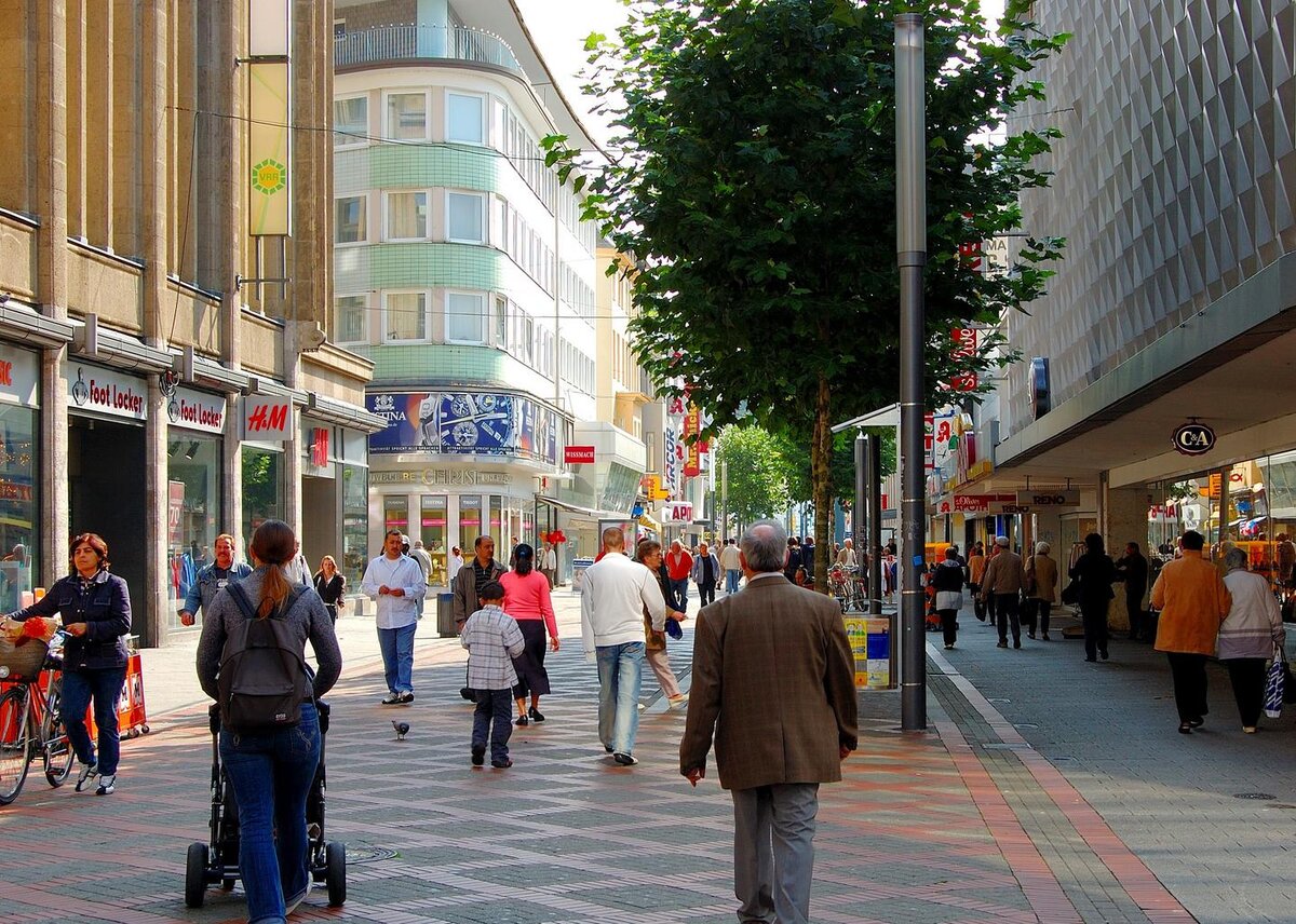
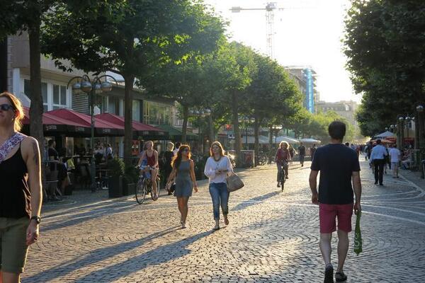
Get an image that contains pedestrians and put it inside a directory somewhere on your computer.
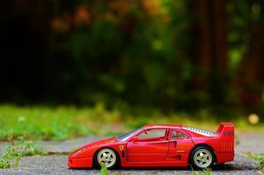
Here are a couple images that I will use as test cases:
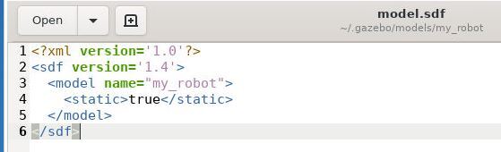
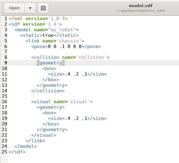
Inside that same directory, write the following code. I will save my file as detect_pedestrians_hog.py:
import cv2 # Import the OpenCV library to enable computer vision

# Author: Addison Sears-Collins
# https://automaticaddison.com
# Description: Detect pedestrians in an image using the
#   Histogram of Oriented Gradients (HOG) method

# Make sure the image file is in the same directory as your code
filename = 'pedestrians_1.jpg'

def main():

  # Create a HOGDescriptor object
  hog = cv2.HOGDescriptor()

  # Initialize the People Detector
  hog.setSVMDetector(cv2.HOGDescriptor_getDefaultPeopleDetector())

  # Load an image
  image = cv2.imread(filename)

  # Detect people
  # image: Source image
  # winStride: step size in x and y direction of the sliding window
  # padding: no. of pixels in x and y direction for padding of sliding window
  # scale: Detection window size increase coefficient
  # bounding_boxes: Location of detected people
  # weights: Weight scores of detected people
  (bounding_boxes, weights) = hog.detectMultiScale(image,
                                                   winStride=(4, 4),
                                                   padding=(8, 8),
                                                   scale=1.05)

  # Draw bounding boxes on the image
  for (x, y, w, h) in bounding_boxes:
    cv2.rectangle(image,
                  (x, y),
                  (x + w, y + h),
                  (0, 0, 255),
                   4)

  # Create the output file name by removing the '.jpg' part
  size = len(filename)
  new_filename = filename[:size - 4]
  new_filename = new_filename + '_detect.jpg'

  # Save the new image in the working directory
  cv2.imwrite(new_filename, image)

  # Display the image
  cv2.imshow("Image", image)

  # Display the window until any key is pressed
  cv2.waitKey(0)

  # Close all windows
  cv2.destroyAllWindows()

main()
Run the code.
python detect_pedestrians_hog.py
Image Results
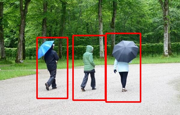
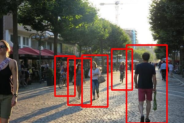
Here is the output for the first image:
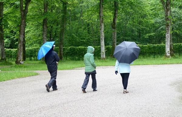
Here is the output for the second image:

Detect Pedestrians in a Video
Now that we know how to detect pedestrians in an image, let’s detect pedestrians in a video.
Find a video file that has pedestrians in it. You can check free video sites like Pixabay if you don’t have any videos.
The video should have dimensions of 1920 x 1080 for this implementation. If you have a video of another size, you will have to tweak the parameters in the code.
Place the video inside a directory.
Now let’s download a library that will apply a fancy mathematical technique called non-maxima suppression to take multiple overlapping bounding boxes and compress them into just one bounding box.
pip install --upgrade imutils
Also, make sure you have NumPy installed, a scientific computing library for Python.
If you’re using Anaconda, you can type:
conda install numpy
Alternatively, you can type:
pip install numpy
Inside that same directory, write the following code. I will save my file as detect_pedestrians_video_hog.py. We will save the output as an .mp4 video file:
# Author: Addison Sears-Collins
# https://automaticaddison.com
# Description: Detect pedestrians in a video using the
#   Histogram of Oriented Gradients (HOG) method

import cv2 # Import the OpenCV library to enable computer vision
import numpy as np # Import the NumPy scientific computing library
from imutils.object_detection import non_max_suppression # Handle overlapping

# Make sure the video file is in the same directory as your code
filename = 'pedestrians_on_street_1.mp4'
file_size = (1920,1080) # Assumes 1920x1080 mp4
scale_ratio = 1 # Option to scale to fraction of original size.

# We want to save the output to a video file
output_filename = 'pedestrians_on_street.mp4'
output_frames_per_second = 20.0

def main():

  # Create a HOGDescriptor object
  hog = cv2.HOGDescriptor()

  # Initialize the People Detector
  hog.setSVMDetector(cv2.HOGDescriptor_getDefaultPeopleDetector())

  # Load a video
  cap = cv2.VideoCapture(filename)

  # Create a VideoWriter object so we can save the video output
  fourcc = cv2.VideoWriter_fourcc(*'mp4v')
  result = cv2.VideoWriter(output_filename,
                           fourcc,
                           output_frames_per_second,
                           file_size)

  # Process the video
  while cap.isOpened():

    # Capture one frame at a time
    success, frame = cap.read()

    # Do we have a video frame? If true, proceed.
    if success:

    	# Resize the frame
      width = int(frame.shape[1] * scale_ratio)
      height = int(frame.shape[0] * scale_ratio)
      frame = cv2.resize(frame, (width, height))

      # Store the original frame
      orig_frame = frame.copy()

      # Detect people
      # image: a single frame from the video
      # winStride: step size in x and y direction of the sliding window
      # padding: no. of pixels in x and y direction for padding of
      #	sliding window
      # scale: Detection window size increase coefficient
      # bounding_boxes: Location of detected people
      # weights: Weight scores of detected people
      # Tweak these parameters for better results
      (bounding_boxes, weights) = hog.detectMultiScale(frame,
                                                       winStride=(16, 16),
                                                       padding=(4, 4),
                                                       scale=1.05)

      # Draw bounding boxes on the frame
      for (x, y, w, h) in bounding_boxes:
            cv2.rectangle(orig_frame,
            (x, y),
            (x + w, y + h),
            (0, 0, 255),
             2)

      # Get rid of overlapping bounding boxes
      # You can tweak the overlapThresh value for better results
      bounding_boxes = np.array([[x, y, x + w, y + h] for (
                                x, y, w, h) in bounding_boxes])

      selection = non_max_suppression(bounding_boxes,
                                      probs=None,
                                      overlapThresh=0.45)

      # draw the final bounding boxes
      for (x1, y1, x2, y2) in selection:
        cv2.rectangle(frame,
                     (x1, y1),
                     (x2, y2),
                     (0, 255, 0),
                      4)

      # Write the frame to the output video file
      result.write(frame)

      # Display the frame
      cv2.imshow("Frame", frame)

      # Display frame for X milliseconds and check if q key is pressed
      # q == quit
      if cv2.waitKey(25) & 0xFF == ord('q'):
        break

    # No more video frames left
    else:
      break

  # Stop when the video is finished
  cap.release()

  # Release the video recording
  result.release()

  # Close all windows
  cv2.destroyAllWindows()

main()
Run the code.
python detect_pedestrians_hog.py
Video Results
Here is a video of the output:


