In this tutorial, we will cover everything you need to know about Extended Kalman Filters (EKF). At the end, I have included a detailed example using Python code to show you how to implement EKFs from scratch.
I recommend going slowly through this tutorial. There is no hurry. There is a lot of new terminology, and I attempt to explain each piece in a simple way, term by term, always referring back to a running example (e.g. a robot car). Try to understand each section in this tutorial before moving on to the next. If something doesn’t make sense, go over it again. By the end of this tutorial, you’ll understand what an EKF is, and you’ll know how to build one starting from nothing but a blank Python program.
Real-World Applications
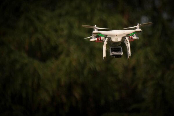
EKFs are common in real-world robotics applications. You’ll see them in everything from self-driving cars to drones.
EKFs are useful when:
- You have a robot with sensors attached to it that enable it to perceive the world.
- Your robot’s sensors are noisy and aren’t 100% accurate (which is always the case).
By running all sensor observations through an EKF, you smooth out noisy sensor measurements and can calculate a better estimate of the state of the robot at each timestep t as the robot moves around in the world. By “state”, I mean “where is the robot,” “what is its orientation,” etc.
Prerequisites
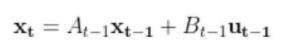
To get the most out of this tutorial, I recommend you go through these two tutorials first. In order to understand what an EKF is, you should know what a state space model and an observation model are. These mathematical models are the two main building blocks for EKFs.
Otherwise, if you feel confident about state space models and observations models, jump right into this tutorial.
What is the Extended Kalman Filter?
Before we dive into the details of how EKFs work, let’s understand what EKFs do on a high level. We want to know why we use EKFs.
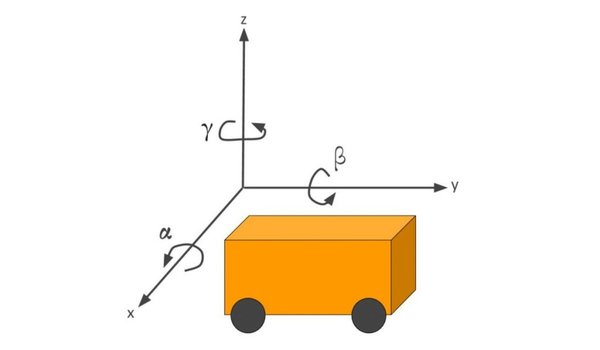
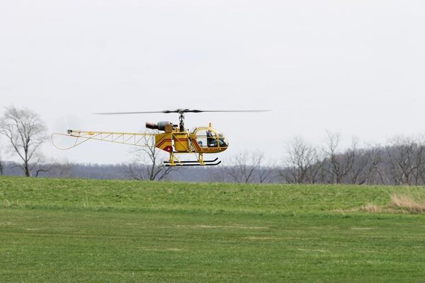
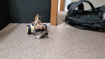
Consider this two-wheeled differential drive robot car below.
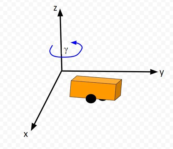
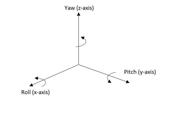
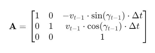
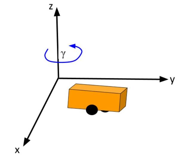
We can model this car like this. The car moves around on the x-y coordinate plane, while the z-axis faces upwards towards the sky:
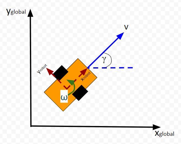
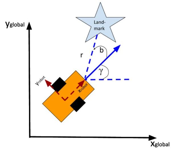
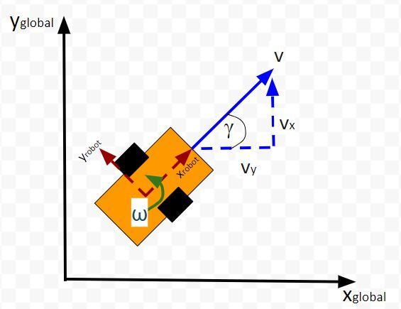
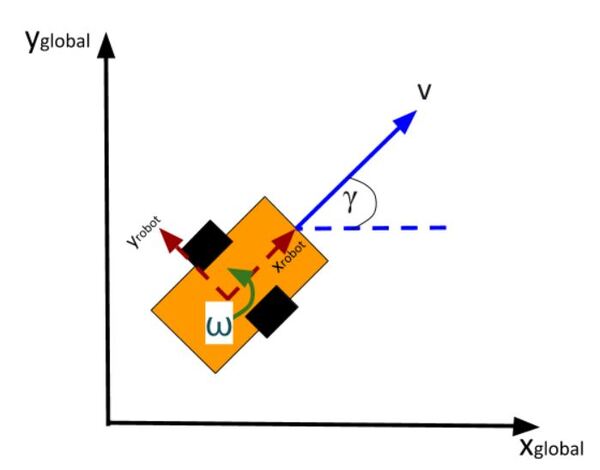
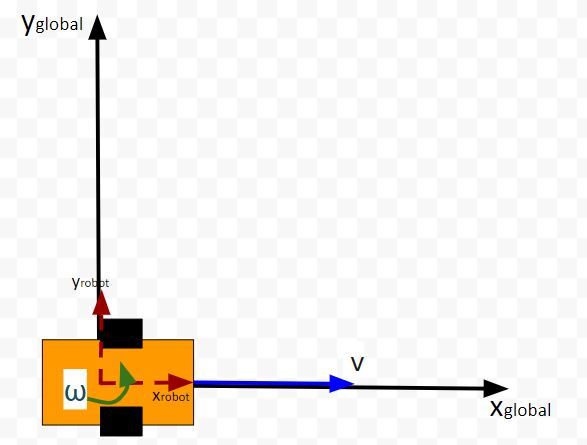
Here is an aerial view of the same robot above. You can see the global coordinate frame, the robot coordinate frame as well as the angular velocity ω (typically in radians per second) and linear velocity v (typically in meters per second):
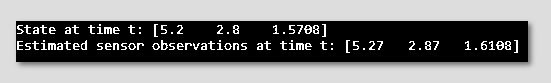
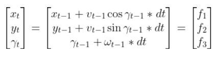
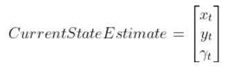
What is this robot’s state at some time t?
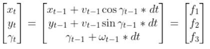
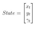
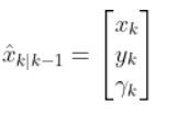
The state of this robot at some time t can be described by just three values: its x position, y position, and yaw angle γ. The yaw angle is the angle of rotation around the z-axis (which points straight out of this page) as measured from the x axis.
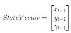
Here is the state vector:
In most cases, the robot has sensors mounted on it. Information from these sensors is used to generate the state vector at each timestep.
However, sensor measurements are uncertain. They aren’t 100% accurate. They can also be noisy, varying a lot from one timestep to the next. So we can never be totally sure where the robot is located in the world and how it is oriented.
Therefore, the state vectors that are calculated at each timestep as the robot moves around in the world is at best an estimate.
How can we generate a better estimate of the state at each timestep t? We don’t want to totally depend on the robot’s sensors to generate an estimate of the state.
Here is what we can do.
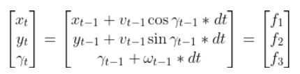
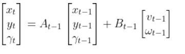
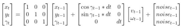
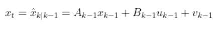
Remember the state space model of the robot car above? Here it is.
You can see that if we know…
- The state estimate for the previous timestep t-1
- The time interval dt from one timestep to the next
- The linear and angular velocity of the car at the previous time step t-1 (i.e. previous control inputs…i.e. commands that were sent to the robot to make the wheels rotate accordingly)
- An estimate of random noise (typically small values…when we send velocity commands to the car, it doesn’t move exactly at those velocities so we add in some random noise)
…then we can estimate the current state of the robot at time t.
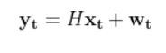
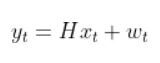
Then, using the observation model, we can use the current state estimate at time t (above) to infer what the corresponding sensor measurement vector would be at the current timestep t (this is the y vector on the left-hand side of the equation below).
From our observation model tutorial, here was the equation:
Note: If that equation above doesn’t make sense to you, please check out the observation model tutorial where I derive it from scratch and show an example in Python code.
The y vector represents predicted sensor measurements for the current timestep t. I say “predicted” because remember the process we went through above. We started by using the previous estimate of the state (at time t-1) to estimate the current state at time t. Then we used the current state at time t to infer what the sensor measurements would be at the current timestep (i.e. y vector).
From here, the Extended Kalman Filter takes care of the rest. It calculates a weighted average of actual sensor measurements at the current timestep t and predicted sensor measurements at the current timestep t to generate a better current state estimate.
The Extended Kalman Filter is an algorithm that leverages our knowledge of the physics of motion of the system (i.e. the state space model) to make small adjustments to (i.e. to filter) the actual sensor measurements (i.e. what the robot’s sensors actually observed) to reduce the amount of noise, and as a result, generate a better estimate of the state of a system.
EKFs tend to generate more accurate estimates of the state (i.e. state vectors) than using just actual sensor measurements alone.
In the case of robotics, EKFs help generate a smooth estimate of the current state of a robotic system over time by combining both actual sensor measurements and predicted sensor measurements to help remove the impact of noise and inaccuracies in sensor measurements.
This is how EKFs work on a high level. I’ll go through the algorithm step by step later in this tutorial.
What is the Difference Between the Kalman Filter and the Extended Kalman Filter?
The regular Kalman Filter is designed to generate estimates of the state just like the Extended Kalman Filter. However, the Kalman Filter only works when the state space model (i.e. state transition function) is linear; that is, the function that governs the transition from one state to the next can be plotted as a line on a graph).
The Extended Kalman Filter was developed to enable the Kalman Filter to be applied to systems that have nonlinear dynamics like our mobile robot.
For example, the Kalman Filter algorithm won’t work with an equation in this form:
But it will work if the equation is in this form:
Another example…consider the equation
Next State = 4 * (Current State) + 3
This is the equation of a line. The regular Kalman Filter can be used on systems like this.
Now, consider this equation
Next State = Current State + 17 * cos(Current State).
This equation is nonlinear. If you were to plot it on a graph, you would see that it is not the graph of a straight line. The regular Kalman Filter won’t work on systems like this. So what do we do?
Fortunately, mathematics can help us linearize nonlinear equations like the one above. Once we linearize this equation, we can then use it in the regular Kalman Filter.
If you were to zoom in to an arbitrary point on a nonlinear curve, you would see that it would look very much like a line. With the Extended Kalman Filter, we convert the nonlinear equation into a linearized form using a special matrix called the Jacobian (see my State Space Model tutorial which shows how to do this). We then use this linearized form of the equation to complete the Kalman Filtering process.
Now let’s take a look at the assumptions behind using EKFs.
Extended Kalman Filter Assumptions
EKFs assume you have already derived two key mathematical equations (i.e. models):
- State Space Model: A state space model (often called the state transition model) is a mathematical equation that helps you estimate the state of a system at time t given the state of a system at time t-1.
- Observation Model: An observation model is a mathematical equation that expresses sensor measurements at time t as a function of the state of a robot at time t.
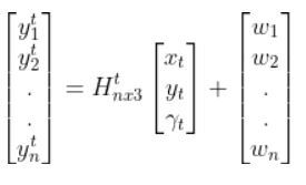
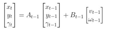
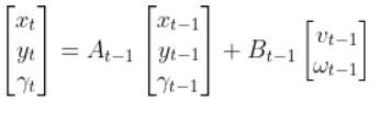
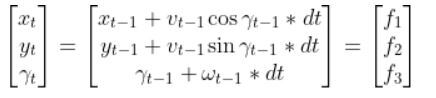
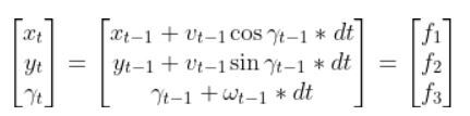
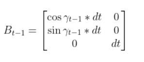
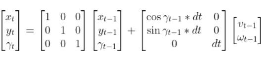
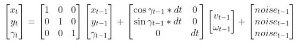
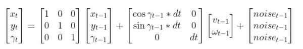
The State Space Model takes the following form:
There is also typically a noise vector term vt-1 added on to the end as well. This noise term is known as process noise. It represents error in the state calculation.
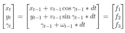
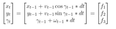
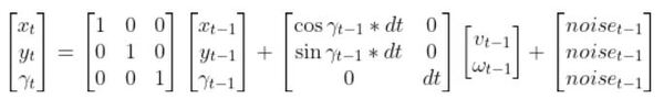
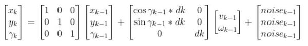
In the robot car example from the state space modeling tutorial, the equation above was expanded out to be:
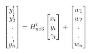
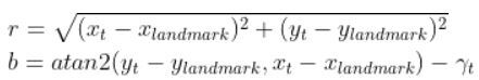
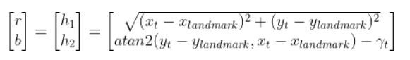
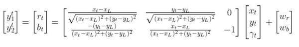
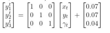
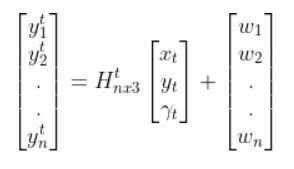
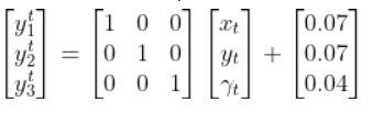
The Observation Model is of the following form:
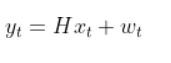
In the robot car example from the observation model tutorial, the equation above was:
Where:
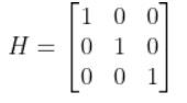
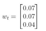
We also assumed that the corresponding noise (error) for our sensor readings was +/-0.07 m for the x position, +/-0.07 m for the y position, and +/-0.04 radians for the yaw angle. Therefore, here was the sensor noise vector:
EKF Algorithm
Overview
On a high-level, the EKF algorithm has two stages, a predict phase and an update (correction phase). Don’t worry if all this sounds confusing. We’ll walk through each line of the EKF algorithm step by step. Each line below corresponds to the same line on this Wikipedia entry on EKFs.
Predict Step
- Using the state space model of the robotics system, predict the state estimate at time t based on the state estimate at time t-1 and the control input applied at time t-1.
- This is exactly what we did in my state space modeling tutorial.
- Predict the state covariance estimate based on the previous covariance and some noise.
Update (Correct) Step
- Calculate the difference between the actual sensor measurements at time t minus what the measurement model predicted the sensor measurements would be for the current timestep t.
- Calculate the measurement residual covariance.
- Calculate the near-optimal Kalman gain.
- Calculate an updated state estimate for time t.
- Update the state covariance estimate for time t.
Let’s go through those bullet points above and define what will likely be some new terms for you.
What Does Covariance Mean?
Note that the covariance measures how much two variables vary with respect to each other.
For example, suppose we have two variables:
X: Number of hours a student spends studying
Y: Course grade
We do some calculations and find that:
Covariance(X,Y) = 147
What does this mean?
A positive covariance means that both variables increase or decrease together. In other words, as the number of hours studying increases, the course grade increases. Similarly, as the number of hours studying decreases, the course grade decreases.
A negative covariance means that while one variable increases, the other variable decreases.
For example, there might be a negative covariance between the number of hours a student spends partying and his course grade.
A covariance of 0 means that the two variables are independent of each other.
For example, a student’s hair color and course grade would have a covariance of 0.
EKF Algorithm Step-by-Step
Let’s walk through each line of the EKF algorithm together, step by step. We will use the notation given on the EKF Wikipedia page where for time they use k instead of t.
Go slowly in this section. There is a lot of new mathematical notation and a lot of subscripts and superscripts. Take your time so that you understand each line of the algorithm. I really want you to finish this article with a strong understanding of EKFs.
1. Initialization
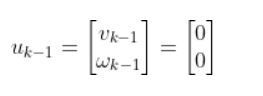
For the first iteration of EKF, we start at time k. In other words, for the first run of EKF, we assume the current time is k.
We initialize the state vector and control vector for the previous time step k-1.
In a real application, the first iteration of EKF, we would let k=1. Therefore, the previous timestep k-1, would be 0.
In our running example of a robotic car, the initial state vector for the previous timestep k-1 would be as follows. Remember the state vector is in terms of the global coordinate frame:
You can see in the equation above that we assume the robot starts out at the origin facing in the positive xglobal direction.
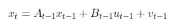
Let’s assume the control input vector at the previous timestep k-1 was nothing (i.e. car was commanded to remain at rest). Therefore, the starting control input vector is as follows.
where:
vk-1 = forward velocity in the robot frame at time k-1
ωk-1 = angular velocity around the z-axis at time k-1 (also known as yaw rate or heading angle)
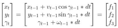
2. Predicted State Estimate

This part of the EKF algorithm is exactly what we did in my state space modeling tutorial.
Remember, we are currently at time k.
We use the state space model, the state estimate for timestep k-1, and the control input vector at the previous time step (e.g. at time k-1) to predict what the state would be for time k (which is the current timestep).
That equation above is the same thing as our equation below. Remember that we used t in my earlier tutorials. However, now I’m replacing t with k to align with the Wikipedia notation for the EKF.
where:
This estimated state prediction for time k is currently our best guess of the current state of the system (e.g. robot).
We also add some noise to the calculation using the process noise vector vk-1 (a 3×1 matrix in the robot car example because we have three states. x position, y position, and yaw angle).
In our running robot car example, we might want to make that noise vector something like [0.01, 0.01, 0.03]. In a real application, you can play around with that number to see what you get.
Robot Car Example
For our running robot car example, let’s see how the Predicted State Estimate step works. Remember dt = dk because t=k…i.e. change in time from one timestep to the next.
We have…
where:
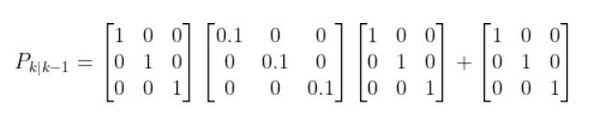
3. Predicted Covariance of the State Estimate

We now have a predicted state estimate for time k, but predicted state estimates aren’t 100% accurate.
In this step—step 3 of the EKF algorithm— we predict the state covariance matrix Pk|k-1 (sometimes called Sigma) for the current time step (i.e. k).
You notice the subscript on P is k|k-1? What this means is that P at timestep k depends on P at timestep k-1.
The symbol “|” means “given”…..P at timestep k “given” the previous timestep k-1.

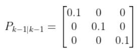
Pk-1|k-1 is a square matrix. It has the same number of rows (and columns) as the number of states in the state vector x.
So, in our example of a robot car with three states [x, y, yaw angle] in the state vector, P (or, commonly, sigma Σ) is a 3×3 matrix. The P matrix has variances on the diagonal and covariances on the off-diagonal.
If terms like variance and covariance don’t make a lot of sense to you, don’t sweat. All you really need to know about P (i.e. Σ in a lot of literature) is that it is a matrix that represents an estimate of the accuracy of the state estimate we made in Step 2.
For the first iteration of EKF, we initialize Pk-1|k-1 to some guessed values (e.g. 0.1 along the diagonal part of the matrix and 0s elsewhere).
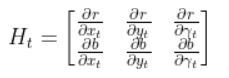
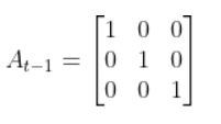
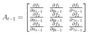
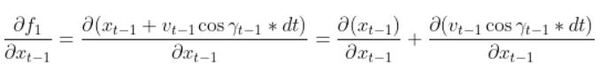
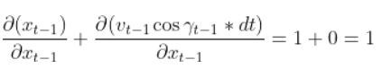
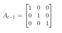
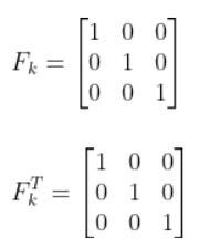
Fk and FkT
In this case, Fk and its transpose FkT are equivalent to At-1 and ATt-1, respectively, from my state space model tutorial.
Recall from my tutorial on state space modeling that the A matrix (F matrix in Wikipedia notation) is a 3×3 matrix (because there are 3 states in our robotic car example) that describes how the state of the system changes from time k-1 to k when no control (i.e. linear and angular velocity) command is executed.
If we had 5 states in our robotic system, the A matrix would be a 5×5 matrix.
Typically, a robot car only drives when the wheels are turning. Therefore, in our running example, Fk (i.e. A) is just the identity matrix and FTk is the transpose of the identity matrix.
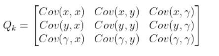
Qk
We have one last term in the predicted covariance of the state equation, Qk. Qk is the state model noise covariance matrix. It is also a 3×3 matrix in our running robot car example because there are three states.
In this case, Q is:
The covariance between two variables that are the same is actually the variance. For example, Cov(x,x) = Variance(x).
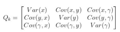
Variance measures the deviation from the mean for points in a single dimension (i.e. x values, y values, or yaw angle values).
For example, suppose Var(x) is a really high number. This means that the x values are all over the place. If Var(x) is low, it means that the x values are clustered around the mean.
The Q term is necessary because states have noise (i.e. they aren’t perfect). Q is sometimes called the “action uncertainty matrix”. When you apply control inputs u at time step k-1 for example, you won’t get an exact value for the Predicted State Estimate at time k (as we calculated in Step 2).
Q represents how much the actual motion deviates from your assumed state space model. It is a square matrix that has the same number of rows and columns as there are states.
We can start by letting Q be the identity matrix and tweak the values through trial and error.
In our running example, Q could be as follows:
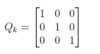
When Q is large, the EKF tracks large changes in the sensor measurements more closely than for smaller Q.
In other words, when Q is large, it means we trust our actual sensor observations more than we trust our predicted sensor measurements from the observation model…more on this later in this tutorial.
Putting the Terms Together
In our running example of the robot car, here would be the equation for the first run through EKF.
This standard form equation:

becomes this after plugging in the values for each of the variables:
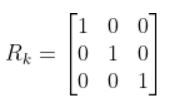
4. Innovation or Measurement Residual

In this step, we calculate the difference between actual sensor observations and predicted sensor observations.
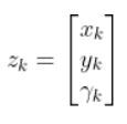
zk is the observation vector. It is a vector of the actual readings from our sensors at time k.
In our running example, suppose that in this case, we have a sensor mounted on our mobile robot that is able to make direct measurements of the three components of the state.
Therefore:
h(x̂k|k-1) is our observation model. It represents the predicted sensor measurements at time k given the predicted state estimate at time k from Step 2. That hat symbol above x means “predicted” or “estimated”.
Recall that the observation model is a mathematical equation that expresses predicted sensor measurements as a function of an estimated state.
This (from the observation model tutorial):
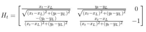
is the exact same thing as this (in Wikipedia notation):
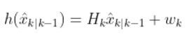
We use the:
- measurement matrix Hk (which is used to convert the predicted state estimate at time k into predicted sensor measurements at time k),
- predicted state estimate x̂k|k-1 that we calculated in Step 2,
- and a sensor noise assumption wk (which is a vector with the same number of elements as there are sensor measurements)
- to calculate h(x̂k|k-1).
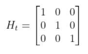
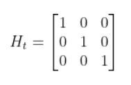
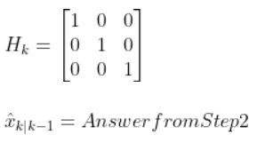
In our running example of the robot car, suppose that in this case, we have a sensor mounted on our mobile robot that is able to make direction measurements of the state [x,y,yaw angle]. In this example, H is the identity matrix. It has the same number of rows as sensor measurements and same number of columns as the number of states) since the state maps 1-to-1 with the sensor measurements.
You can find wk by looking at the sensor error which should be on the datasheet that comes with the sensor when you purchase it online or from the store. If you are unsure what to put for the sensor noise, just put some random (low) values.
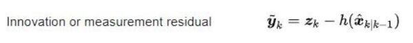
In our running example, we have a sensor that can directly sense the three states. I’ll set the sensor noise for each of the three measurements as follows:
You now have everything you need to calculate the innovation residual ỹ using this equation:
5. Innovation (or residual) Covariance

In this step, we:
- use the predicted covariance of the state estimate Pk|k-1 from Step 3
- and the measurement matrix Hk and its transpose.
- and Rk (sensor measurement noise covariance matrix…which is a covariance matrix that has the same number of rows as sensor measurements and same number of columns as sensor measurements)
- to calculate Sk, which represents the measurement residual covariance (also known as measurement prediction covariance).
I like to start out by making Rk the identity matrix. You can then tweak it through trial and error.
If we are sure about our sensor measurements, the values along the diagonal of R decrease to zero.
You now have all the values you need to calculate Sk:

6. Near-optimal Kalman Gain

We use:
- the Predicted Covariance of the State Estimate from Step 3,
- the measurement matrix Hk,
- and Sk from Step 5
- to calculate the Kalman gain Kk
K indicates how much the state and covariance of the state predictions should be corrected (see Steps 7 and 8 below) as a result of the new actual sensor measurements (zk).
If sensor measurement noise is large, then K approaches 0, and sensor measurements will be mostly ignored.
If prediction noise (using the dynamical model/physics of the system) is large, then K approaches 1, and sensor measurements will dominate the estimate of the state [x,y,yaw angle].
7. Updated State Estimate

In this step, we calculate an updated (corrected) state estimate based on the values from:
- Step 2 (predicted state estimate for current time step k),
- Step 6 (near-optimal Kalman gain from 6),
- and Step 4 (measurement residual).
This step answers the all-important question: What is the state of the robotic system after seeing the new sensor measurement? It is our best estimate for the state of the robotic system at the current timestep k.
8. Updated Covariance of the State Estimate
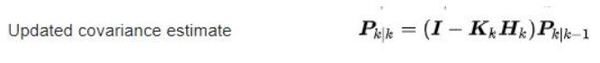
In this step, we calculate an updated (corrected) covariance of the state estimate based on the values from:
- Step 3 (predicted covariance of the state estimate for current time step k),
- Step 6 (near-optimal Kalman gain from 6),
- measurement matrix Hk.
This step answers the question: What is the covariance of the state of the robotic system after seeing the fresh sensor measurements?
Python Code for the Extended Kalman Filter
Let’s put all we have learned into code. Here is an example Python implementation of the Extended Kalman Filter. The method takes an observation vector zk as its parameter and returns an updated state and covariance estimate.
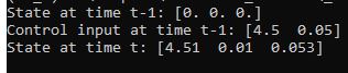
Let’s assume our robot starts out at the origin (x=0, y=0), and the yaw angle is 0 radians.
We then apply a forward linear velocity v of 4.5 meters per second at time k-1 and an angular velocity ω of 0 radians per second.
At each timestep k, we take a fresh observation (zk).
The code below goes through 5 timesteps (i.e. we go from k=1 to k=5). We assume the time interval between each timestep is 1 second (i.e. dk=1).
Here is our series of sensor observations at each of the 5 timesteps…k=1 to k=5 [x,y,yaw angle]:
- k=1: [4.721,0.143,0.006]
- k=2: [9.353,0.284,0.007]
- k=3: [14.773,0.422,0.009]
- k=4: [18.246,0.555,0.011]
- k=5: [22.609,0.715,0.012]
Here is the code:
import numpy as np
# Author: Addison Sears-Collins
# https://automaticaddison.com
# Description: Extended Kalman Filter example (two-wheeled mobile robot)
# Supress scientific notation when printing NumPy arrays
np.set_printoptions(precision=3,suppress=True)
# A matrix
# 3x3 matrix -> number of states x number of states matrix
# Expresses how the state of the system [x,y,yaw] changes
# from k-1 to k when no control command is executed.
# Typically a robot on wheels only drives when the wheels are told to turn.
# For this case, A is the identity matrix.
# A is sometimes F in the literature.
A_k_minus_1 = np.array([[1.0, 0, 0],
[ 0,1.0, 0],
[ 0, 0, 1.0]])
# Noise applied to the forward kinematics (calculation
# of the estimated state at time k from the state
# transition model of the mobile robot). This is a vector
# with the number of elements equal to the number of states
process_noise_v_k_minus_1 = np.array([0.01,0.01,0.003])
# State model noise covariance matrix Q_k
# When Q is large, the Kalman Filter tracks large changes in
# the sensor measurements more closely than for smaller Q.
# Q is a square matrix that has the same number of rows as states.
Q_k = np.array([[1.0, 0, 0],
[ 0, 1.0, 0],
[ 0, 0, 1.0]])
# Measurement matrix H_k
# Used to convert the predicted state estimate at time k
# into predicted sensor measurements at time k.
# In this case, H will be the identity matrix since the
# estimated state maps directly to state measurements from the
# odometry data [x, y, yaw]
# H has the same number of rows as sensor measurements
# and same number of columns as states.
H_k = np.array([[1.0, 0, 0],
[ 0,1.0, 0],
[ 0, 0, 1.0]])
# Sensor measurement noise covariance matrix R_k
# Has the same number of rows and columns as sensor measurements.
# If we are sure about the measurements, R will be near zero.
R_k = np.array([[1.0, 0, 0],
[ 0, 1.0, 0],
[ 0, 0, 1.0]])
# Sensor noise. This is a vector with the
# number of elements equal to the number of sensor measurements.
sensor_noise_w_k = np.array([0.07,0.07,0.04])
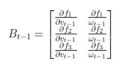
def getB(yaw, deltak):
"""
Calculates and returns the B matrix
3x2 matix -> number of states x number of control inputs
The control inputs are the forward speed and the
rotation rate around the z axis from the x-axis in the
counterclockwise direction.
[v,yaw_rate]
Expresses how the state of the system [x,y,yaw] changes
from k-1 to k due to the control commands (i.e. control input).
:param yaw: The yaw angle (rotation angle around the z axis) in rad
:param deltak: The change in time from time step k-1 to k in sec
"""
B = np.array([ [np.cos(yaw)*deltak, 0],
[np.sin(yaw)*deltak, 0],
[0, deltak]])
return B
def ekf(z_k_observation_vector, state_estimate_k_minus_1,
control_vector_k_minus_1, P_k_minus_1, dk):
"""
Extended Kalman Filter. Fuses noisy sensor measurement to
create an optimal estimate of the state of the robotic system.
INPUT
:param z_k_observation_vector The observation from the Odometry
3x1 NumPy Array [x,y,yaw] in the global reference frame
in [meters,meters,radians].
:param state_estimate_k_minus_1 The state estimate at time k-1
3x1 NumPy Array [x,y,yaw] in the global reference frame
in [meters,meters,radians].
:param control_vector_k_minus_1 The control vector applied at time k-1
3x1 NumPy Array [v,v,yaw rate] in the global reference frame
in [meters per second,meters per second,radians per second].
:param P_k_minus_1 The state covariance matrix estimate at time k-1
3x3 NumPy Array
:param dk Time interval in seconds
OUTPUT
:return state_estimate_k near-optimal state estimate at time k
3x1 NumPy Array ---> [meters,meters,radians]
:return P_k state covariance_estimate for time k
3x3 NumPy Array
"""
######################### Predict #############################
# Predict the state estimate at time k based on the state
# estimate at time k-1 and the control input applied at time k-1.
state_estimate_k = A_k_minus_1 @ (
state_estimate_k_minus_1) + (
getB(state_estimate_k_minus_1[2],dk)) @ (
control_vector_k_minus_1) + (
process_noise_v_k_minus_1)
print(f'State Estimate Before EKF={state_estimate_k}')
# Predict the state covariance estimate based on the previous
# covariance and some noise
P_k = A_k_minus_1 @ P_k_minus_1 @ A_k_minus_1.T + (
Q_k)
################### Update (Correct) ##########################
# Calculate the difference between the actual sensor measurements
# at time k minus what the measurement model predicted
# the sensor measurements would be for the current timestep k.
measurement_residual_y_k = z_k_observation_vector - (
(H_k @ state_estimate_k) + (
sensor_noise_w_k))
print(f'Observation={z_k_observation_vector}')
# Calculate the measurement residual covariance
S_k = H_k @ P_k @ H_k.T + R_k
# Calculate the near-optimal Kalman gain
# We use pseudoinverse since some of the matrices might be
# non-square or singular.
K_k = P_k @ H_k.T @ np.linalg.pinv(S_k)
# Calculate an updated state estimate for time k
state_estimate_k = state_estimate_k + (K_k @ measurement_residual_y_k)
# Update the state covariance estimate for time k
P_k = P_k - (K_k @ H_k @ P_k)
# Print the best (near-optimal) estimate of the current state of the robot
print(f'State Estimate After EKF={state_estimate_k}')
# Return the updated state and covariance estimates
return state_estimate_k, P_k
def main():
# We start at time k=1
k = 1
# Time interval in seconds
dk = 1
# Create a list of sensor observations at successive timesteps
# Each list within z_k is an observation vector.
z_k = np.array([[4.721,0.143,0.006], # k=1
[9.353,0.284,0.007], # k=2
[14.773,0.422,0.009],# k=3
[18.246,0.555,0.011], # k=4
[22.609,0.715,0.012]])# k=5
# The estimated state vector at time k-1 in the global reference frame.
# [x_k_minus_1, y_k_minus_1, yaw_k_minus_1]
# [meters, meters, radians]
state_estimate_k_minus_1 = np.array([0.0,0.0,0.0])
# The control input vector at time k-1 in the global reference frame.
# [v, yaw_rate]
# [meters/second, radians/second]
# In the literature, this is commonly u.
# Because there is no angular velocity and the robot begins at the
# origin with a 0 radians yaw angle, this robot is traveling along
# the positive x-axis in the global reference frame.
control_vector_k_minus_1 = np.array([4.5,0.0])
# State covariance matrix P_k_minus_1
# This matrix has the same number of rows (and columns) as the
# number of states (i.e. 3x3 matrix). P is sometimes referred
# to as Sigma in the literature. It represents an estimate of
# the accuracy of the state estimate at time k made using the
# state transition matrix. We start off with guessed values.
P_k_minus_1 = np.array([[0.1, 0, 0],
[ 0,0.1, 0],
[ 0, 0, 0.1]])
# Start at k=1 and go through each of the 5 sensor observations,
# one at a time.
# We stop right after timestep k=5 (i.e. the last sensor observation)
for k, obs_vector_z_k in enumerate(z_k,start=1):
# Print the current timestep
print(f'Timestep k={k}')
# Run the Extended Kalman Filter and store the
# near-optimal state and covariance estimates
optimal_state_estimate_k, covariance_estimate_k = ekf(
obs_vector_z_k, # Most recent sensor measurement
state_estimate_k_minus_1, # Our most recent estimate of the state
control_vector_k_minus_1, # Our most recent control input
P_k_minus_1, # Our most recent state covariance matrix
dk) # Time interval
# Get ready for the next timestep by updating the variable values
state_estimate_k_minus_1 = optimal_state_estimate_k
P_k_minus_1 = covariance_estimate_k
# Print a blank line
print()
# Program starts running here with the main method
main()
Take a closer look at the output. You can see how much the EKF helps us smooth noisy sensor measurements.
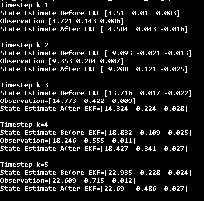
For example, notice at timestep k=3 that our state space model predicted the following:
[x=13.716 meters, y=0.017 meters, yaw angle = -0.022 radians]
The observation from the sensor mounted on the robot was:
[x=14.773 meters, y=0.422 meters, yaw angle = 0.009 radians]
Oops! Looks like our sensors are indicating that our state space model underpredicted all state values.
This is where the EKF helped us. We use EKF to blend the estimated state value with the sensor data (which we don’t trust 100% but we do trust some) to create a better state estimate of:
[x=14.324 meters, y=0.224 meters, yaw angle = -0.028 radians]
And voila! There you have it.
Conclusion
The Extended Kalman Filter is a powerful mathematical tool if you:
- Have a state space model of how the system behaves,
- Have a stream of sensor observations about the system,
- Can represent uncertainty in the system (inaccuracies and noise in the state space model and in the sensor data)
- You can merge actual sensor observations with predictions to create a good estimate of the state of a robotic system.
That’s it for the EKF. You now know what all those weird mathematical symbols mean, and hopefully the EKF is no longer intimidating to you (it definitely was to me when I first learned about EKFs).
What I’ve provided to you in this tutorial is an EKF for a simple two-wheeled mobile robot, but you can expand the EKF to any system you can appropriately model. In fact, the Extended Kalman Filter was used in the onboard guidance and navigation system for the Apollo spacecraft missions.
Feel free to return to this tutorial any time in the future when you’re confused about the Extended Kalman Filter.
Keep building!
Further Reading
If you want to dive deeper into Kalman Filters, check out this free book on GitHub by Roger Labbe.