*** This tutorial is two years old and may no longer work properly. You can find an updated tutorial for object recognition at this link***
In this tutorial, we will develop a program that can recognize objects in a real-time video stream on a built-in laptop webcam using deep learning.
Object recognition involves two main tasks:
- Object Detection (Where are the objects?): Locate objects in a photo or video frame
- Image Classification (What are the objects?): Predict the type of each object in a photo or video frame
Humans can do both tasks effortlessly, but computers cannot.
Computers require a lot of processing power to take full advantage of the state-of-the-art algorithms that enable object recognition in real time. However, in recent years, the technology has matured, and real-time object recognition is now possible with only a laptop computer and a webcam.
Real-time object recognition systems are currently being used in a number of real-world applications, including the following:
- Self-driving cars: detection of pedestrians, cars, traffic lights, bicycles, motorcycles, trees, sidewalks, etc.
- Surveillance: catching thieves, counting people, identifying suspicious behavior, child detection.
- Traffic monitoring: identifying traffic jams, catching drivers that are breaking the speed limit.
- Security: face detection, identity verification on a smartphone.
- Robotics: robotic surgery, agriculture, household chores, warehouses, autonomous delivery.
- Sports: ball tracking in baseball, golf, and football.
- Agriculture: disease detection in fruits.
- Food: food identification.
There are a lot of steps in this tutorial. Have fun, be patient, and be persistent. Don’t give up! If something doesn’t work the first time around, try again. You will learn a lot more by fighting through to the end of this project. Stay relentless!
By the end of this tutorial, you will have the rock-solid confidence to detect and recognize objects in real time on your laptop’s GPU (Graphics Processing Unit) using deep learning.
Let’s get started!
Table of Contents
- You Will Need
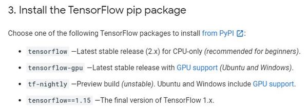
- Install TensorFlow CPU
- Install TensorFlow GPU
- –Install CUDA Toolkit v9.0
- –Install the NVIDIA CUDA Deep Neural Network library (cuDNN)
- –Install TensorFlow GPU
- –Install TensorFlow Models
- –Install Protobuf
- –Install COCO API
- –Test the Installation
- Install LabelImg
- Recognize Objects Using Your WebCam
- –Approach
- –Implementation (Python Code)
You Will Need
Install TensorFlow CPU
We need to get all the required software set up on our computer. I will be following this really helpful tutorial.
Open an Anaconda command prompt terminal.
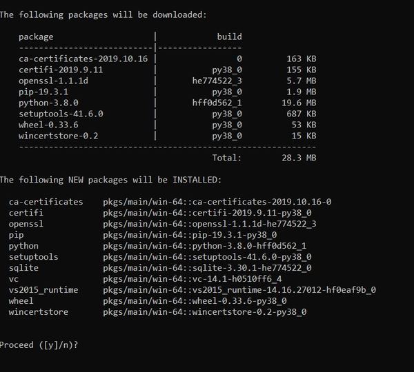
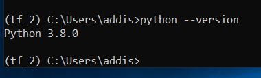
Type the command below to create a virtual environment named tensorflow_cpu that has Python 3.6 installed.
conda create -n tensorflow_cpu pip python=3.6
Press y and then ENTER.
A virtual environment is like an independent Python workspace which has its own set of libraries and Python version installed. For example, you might have a project that needs to run using an older version of Python, like Python 2.7. You might have another project that requires Python 3.7. You can create separate virtual environments for these projects.
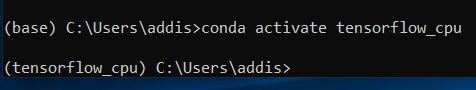
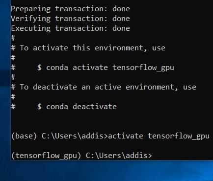
Now, let’s activate the virtual environment by using this command:
conda activate tensorflow_cpu
Type the following command to install TensorFlow CPU.
pip install --ignore-installed --upgrade tensorflow==1.9
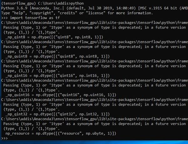
Wait for Tensorflow CPU to finish installing. Once it is finished installing, launch Python by typing the following command:
python

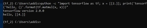
Type:
import tensorflow as tf
Here is what my screen looks like now:
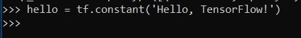
Now type the following:
hello = tf.constant('Hello, TensorFlow!')
sess = tf.Session()
You should see a message that says: “Your CPU supports instructions that this TensorFlow binary….”. Just ignore that. Your TensorFlow will still run fine.
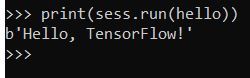
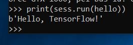
Now run this command to complete the test of the installation:
print(sess.run(hello))
Press CTRL+Z. Then press ENTER to exit.
Type:
exit
That’s it for TensorFlow CPU. Now let’s install TensorFlow GPU.
Install TensorFlow GPU
Your system must have the following requirements:
- Nvidia GPU (GTX 650 or newer…I’ll show you later how to find out what Nvidia GPU version is in your computer)
- CUDA Toolkit v9.0 (we will install this later in this tutorial)
- CuDNN v7.0.5 (we will install this later in this tutorial)
- Anaconda with Python 3.7+
Here is a good tutorial that walks through the installation, but I’ll outline all the steps below.
Install CUDA Toolkit v9.0
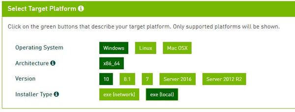
The first thing we need to do is to install the CUDA Toolkit v9.0. Go to this link.
Select your operating system. In my case, I will select Windows, x86_64, Version 10, and exe (local).
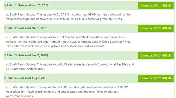
Download the Base Installer as well as all the patches. I downloaded all these files to my Desktop. It will take a while to download, so just wait while your computer downloads everything.
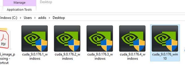
Open the folder where the downloads were saved to.
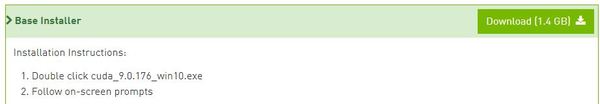
Double-click on the Base Installer program, the largest of the files that you downloaded from the website.
Click Yes to allow the program to make changes to your device.
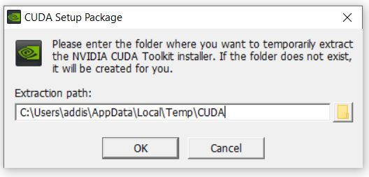
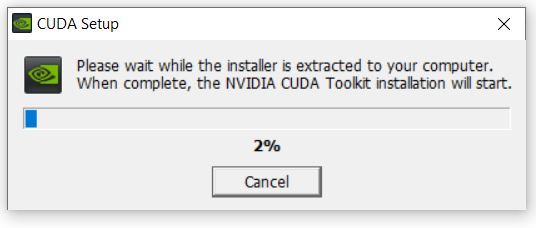
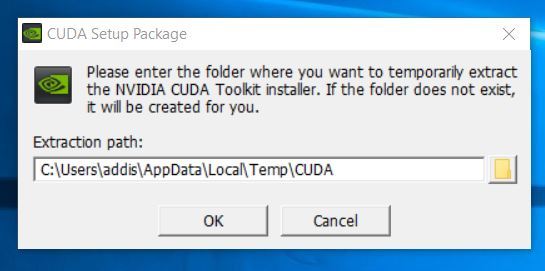
Click OK to extract the files to your computer.
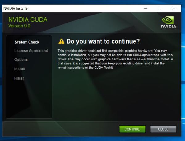
I saw this error window. Just click Continue.
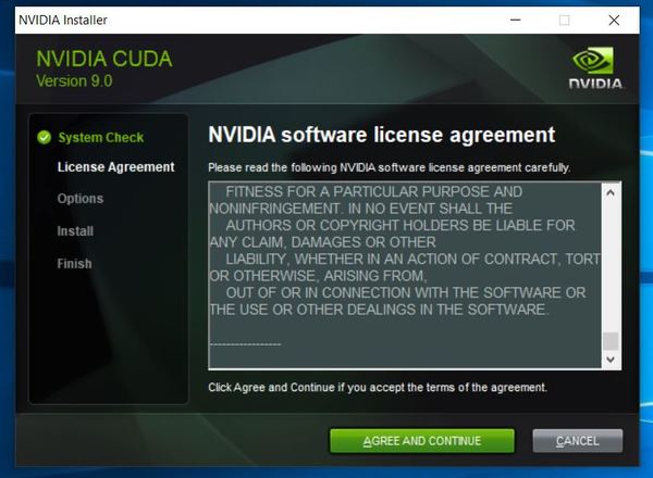
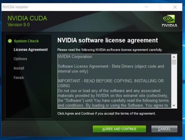
Click Agree and Continue.
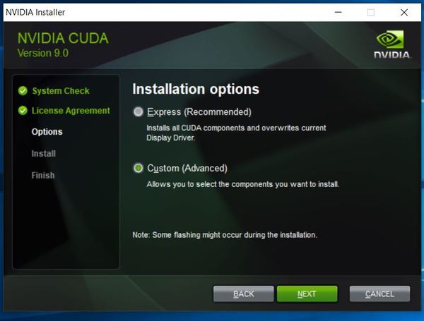
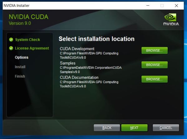
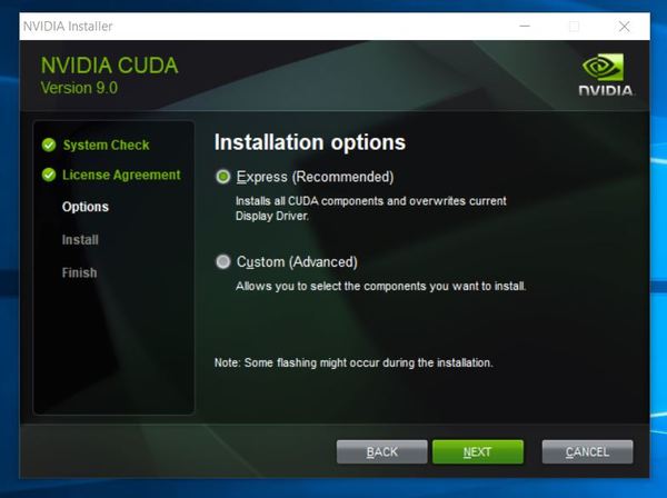
If you saw that error window earlier… “…you may not be able to run CUDA applications with this driver…,” select the Custom (Advanced) install option and click Next. Otherwise, do the Express installation and follow all the prompts.
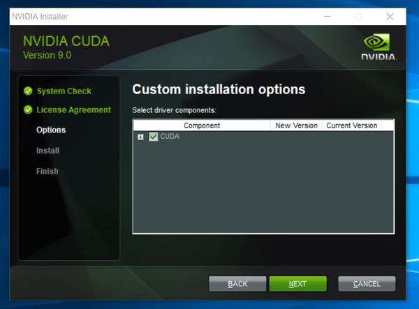
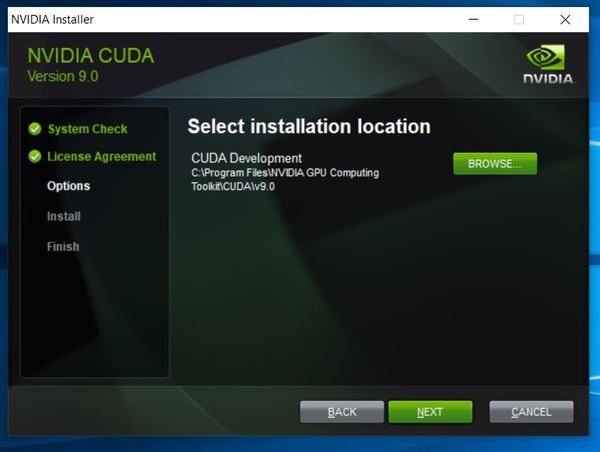
Uncheck the Driver components, PhysX, and Visual Studio Integration options. Then click Next.
Click Next.
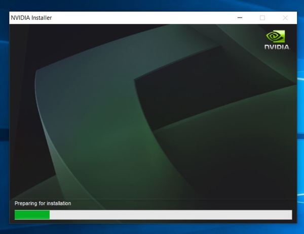
Wait for everything to install.
Click Close.
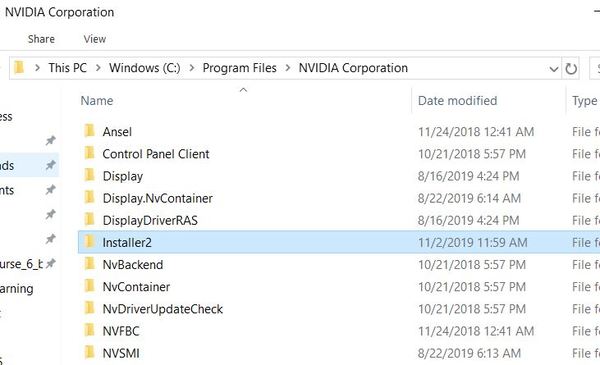
Delete C:\Program Files\NVIDIA Corporation\Installer2.
Double-click on Patch 1.
Click Yes to allow changes to your computer.
Click OK.
Click Agree and Continue.
Go to Custom (Advanced) and click Next.
Click Next.
Click Close.
The process is the same for Patch 2. Double-click on Patch 2 now.
Click Yes to allow changes to your computer.
Click OK.
Click Agree and Continue.
Go to Custom (Advanced) and click Next.
Click Next.
Click Close.
The process is the same for Patch 3. Double-click on Patch 3 now.
Click Yes to allow changes to your computer.
Click OK.
Click Agree and Continue.
Go to Custom (Advanced) and click Next.
Click Next.
Click Close.
The process is the same for Patch 4. Double-click on Patch 4 now.
Click Yes to allow changes to your computer.
Click OK.
Click Agree and Continue.
Go to Custom (Advanced) and click Next.
Click Next.
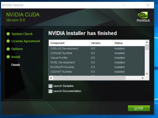
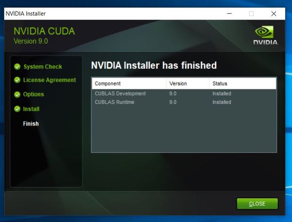
After you’ve installed Patch 4, your screen should look like this:
Click Close.
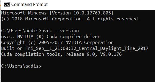
To verify your CUDA installation, go to the command terminal on your computer, and type:
nvcc --version
Install the NVIDIA CUDA Deep Neural Network library (cuDNN)
Now that we installed the CUDA 9.0 base installer and its four patches, we need to install the NVIDIA CUDA Deep Neural Network library (cuDNN). Official instructions for installing are on this page, but I’ll walk you through the process below.
Go to https://developer.nvidia.com/rdp/cudnn-download
Create a user profile if needed and log in.

Go to this page: https://developer.nvidia.com/rdp/cudnn-download
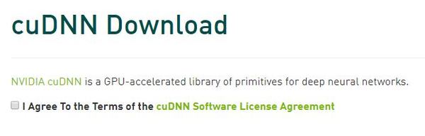
Agree to the terms of the cuDNN Software License Agreement.
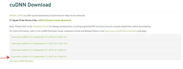
We have CUDA 9.0, so we need to click cuDNN v7.6.4 (September 27, 2019), for CUDA 9.0.
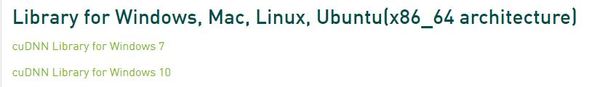
I have Windows 10, so I will download cuDNN Library for Windows 10.
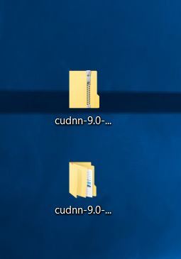
In my case, the zip file downloaded to my Desktop. I will unzip that zip file now, which will create a new folder of the same name…just without the .zip part. These are your cuDNN files. We’ll come back to these in a second.
Before we get going, let’s double check what GPU we have. If you are on a Windows machine, search for the “Device Manager.”
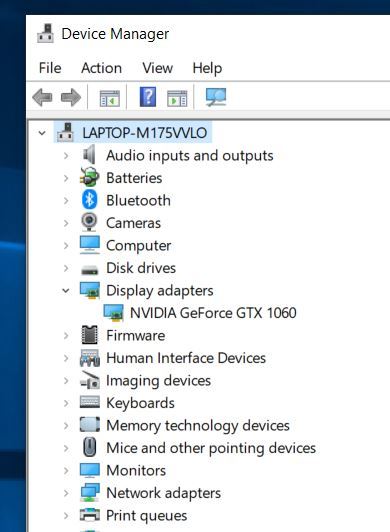
Once you have the Device Manager open, you should see an option near the top for “Display Adapters.” Click the drop-down arrow next to that, and you should see the name of your GPU. Mine is NVIDIA GeForce GTX 1060.
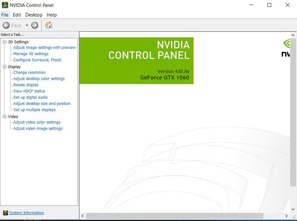
If you are on Windows, you can also check what NVIDIA graphics driver you have by right-clicking on your Desktop and clicking the NVIDIA Control Panel. My version is 430.86. This version fits the requirements for cuDNN.
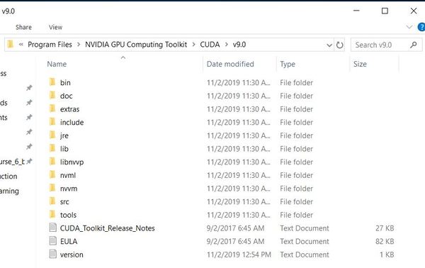
Ok, now that we have verified that our system meets the requirements, lets navigate to C:\Program Files\NVIDIA GPU Computing Toolkit\CUDA\v9.0, your CUDA Toolkit directory.
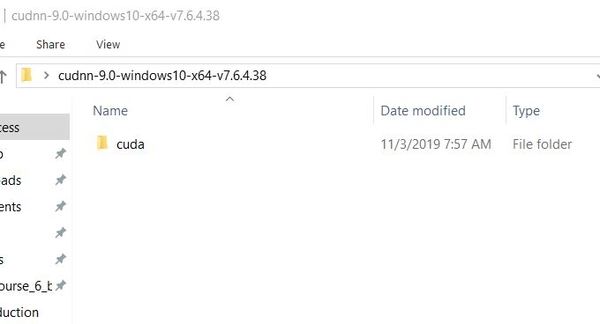
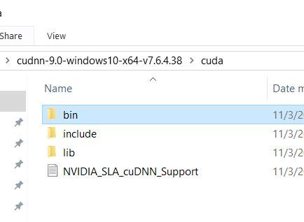
Now go to your cuDNN files, that new folder that was created when you did the unzipping. Inside that folder, you should see a folder named cuda. Click on it.
Click bin.
Copy cudnn64_7.dll to C:\Program Files\NVIDIA GPU Computing Toolkit\CUDA\v9.0\bin. Your computer might ask you to allow Administrative Privileges. Just click Continue when you see that prompt.
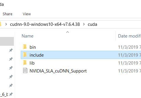
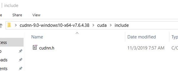
Now go back to your cuDNN files. Inside the cuda folder, click on include. You should see a file named cudnn.h.
Copy that file to C:\Program Files\NVIDIA GPU Computing Toolkit\CUDA\v9.0\include. Your computer might ask you to allow Administrative Privileges. Just click Continue when you see that prompt.
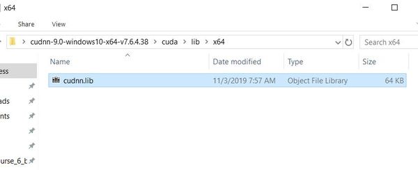
Now go back to your cuDNN files. Inside the cuda folder, click on lib -> x64. You should see a file named cudnn.lib.
Copy that file to C:\Program Files\NVIDIA GPU Computing Toolkit\CUDA\v9.0\lib\x64. Your computer might ask you to allow Administrative Privileges. Just click Continue when you see that prompt.
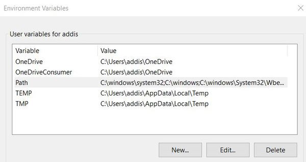
If you are using Windows, do a search on your computer for Environment Variables. An option should pop up to allow you to edit the Environment Variables on your computer.
Click on Environment Variables.
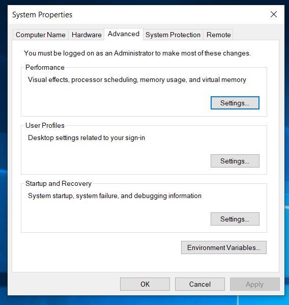
Make sure you CUDA_PATH variable is set to C:\Program Files\NVIDIA GPU Computing Toolkit\CUDA\v9.0.
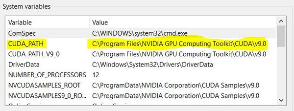
I recommend restarting your computer now.
Install TensorFlow GPU
Now we need to install TensorFlow GPU. Open a new Anaconda terminal window.
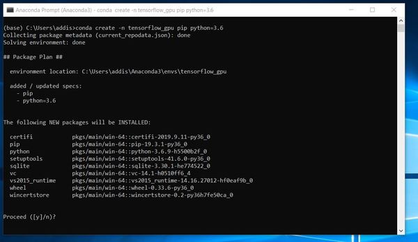
Create a new Conda virtual environment named tensorflow_gpu by typing this command:
conda create -n tensorflow_gpu pip python=3.6
Type y and press Enter.
Activate the virtual environment.
conda activate tensorflow_gpu
Install TensorFlow GPU for Python.
pip install --ignore-installed --upgrade tensorflow-gpu==1.9
Wait for TensorFlow GPU to install.
Now let’s test the installation. Launch the Python interpreter.
python
Type this command.
import tensorflow as tf
If you don’t see an error, TensorFlow GPU is successfully installed.
Now type this:
hello = tf.constant('Hello, TensorFlow!')
And run this command. It might take a few minutes to run, so just wait until it finishes:
sess = tf.Session()
Now type this command to complete the test of the installation:
print(sess.run(hello))
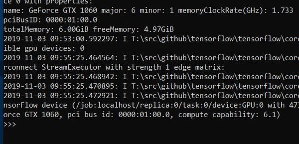
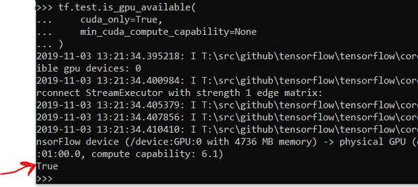
You can further confirm whether TensorFlow can access the GPU, by typing the following into the Python interpreter (just copy and paste into the terminal window while the Python interpreter is running).
tf.test.is_gpu_available(
    cuda_only=True,
    min_cuda_compute_capability=None
)
To exit the Python interpreter, type:
exit()
And press Enter.
Install TensorFlow Models
Now that we have everything setup, let’s install some useful libraries. I will show you the steps for doing this in my TensorFlow GPU virtual environment, but the steps are the same for the TensorFlow CPU virtual environment.
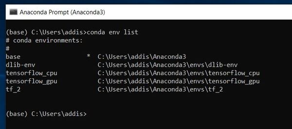
Open a new Anaconda terminal window. Let’s take a look at the list of virtual environments that we can activate.
conda env list
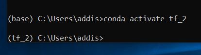
I’m going to activate the TensorFlow GPU virtual environment.
conda activate tensorflow_gpu
Install the libraries. Type this command:
conda install pillow lxml jupyter matplotlib opencv cython
Press y to proceed.
Once that is finished, you need to create a folder somewhere that has the TensorFlow Models (e.g. C:\Users\addis\Documents\TensorFlow). If you have a D drive, you can also save it there as well.
In your Anaconda terminal window, move to the TensorFlow directory you just created. You will use the cd command to change to that directory. For example:
cd C:\Users\addis\Documents\TensorFlow
Go to the TensorFlow models page on GitHub: https://github.com/tensorflow/models.
Click the button to download the zip file of the repository. It is a large file, so it will take a while to download.
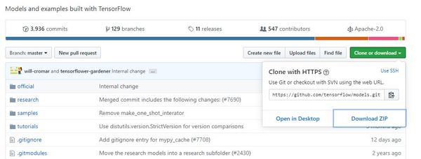
Move the zip folder to the TensorFlow directory you created earlier and extract the contents.
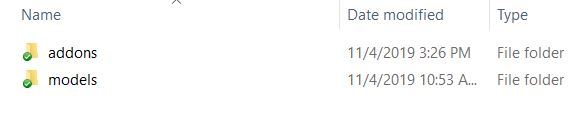
Rename the extracted folder to models instead of models-master. Your TensorFlow directory hierarchy should look like this:
TensorFlow
- models
- official
- research
- samples
- tutorials
Install Protobuf
Now we need to install Protobuf, which is used by the TensorFlow Object Detection API to configure the training and model parameters.
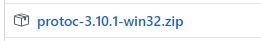
Go to this page: https://github.com/protocolbuffers/protobuf/releases
Download the latest *-win32.zip release (assuming you are on a Windows machine).
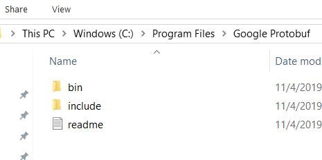
Create a folder in C:\Program Files named it Google Protobuf.
Extract the contents of the downloaded *-win32.zip, inside C:\Program Files\Google Protobuf
Search for Environment Variables on your system. A window should pop up that says System Properties.
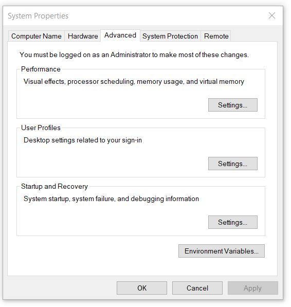
Click Environment Variables.
Go down to the Path variable and click Edit.
Click New.
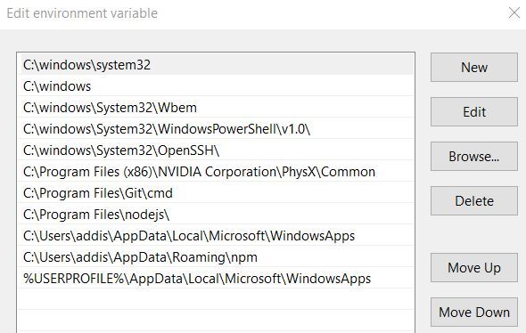
Add C:\Program Files\Google Protobuf\bin
You can also add it the Path System variable.
Click OK a few times to close out all the windows.
Open a new Anaconda terminal window.
I’m going to activate the TensorFlow GPU virtual environment.
conda activate tensorflow_gpu
cd into your \TensorFlow\models\research\ directory and run the following command:
for /f %i in ('dir /b object_detection\protos\*.proto') do protoc object_detection\protos\%i --python_out=.
Now go back to the Environment Variables on your system. Create a New Environment Variable named PYTHONPATH (if you don’t have one already). Replace C:\Python27amd64 if you don’t have Python installed there. Also, replace <your_path> with the path to your TensorFlow folder.
C:\Python27amd64;C:\<your_path>\TensorFlow\models\research\object_detection
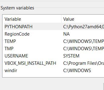
For example:
C:\Python27amd64;C:\Users\addis\Documents\TensorFlow
Now add these two paths to your PYTHONPATH environment variable:
C:\<your_path>\TensorFlow\models\research\
C:\<your_path>\TensorFlow\models\research\slim
Install COCO API
Now, we are going to install the COCO API. You don’t need to worry about what this is at this stage. I’ll explain it later.
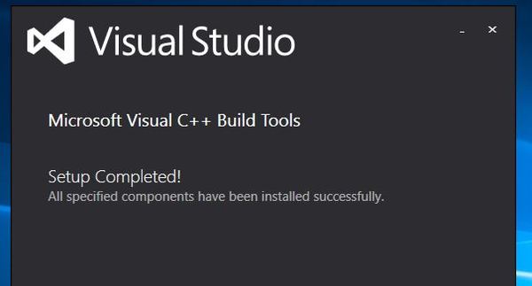
Download the Visual Studios Build Tools here: Visual C++ 2015 build tools from here: https://go.microsoft.com/fwlink/?LinkId=691126
Choose the default installation.
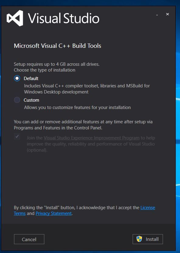
After it has installed, restart your computer.
Open a new Anaconda terminal window.
I’m going to activate the TensorFlow GPU virtual environment.
conda activate tensorflow_gpu
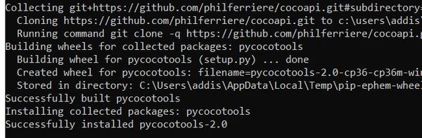
cd into your \TensorFlow\models\research\ directory and run the following command to install pycocotools (everything below goes on one line):
pip install git+https://github.com/philferriere/cocoapi.git#subdirectory=PythonAPI
If it doesn’t work, install git: https://git-scm.com/download/win
Follow all the default settings for installing Git. You will have to click Next several times.
Once you have finished installing Git, run this command (everything goes on one line):
pip install git+https://github.com/philferriere/cocoapi.git#subdirectory=PythonAPI
Test the Installation
Open a new Anaconda terminal window.
I’m going to activate the TensorFlow GPU virtual environment.
conda activate tensorflow_gpu
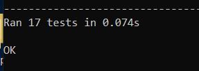
cd into your \TensorFlow\models\research\object_detection\builders directory and run the following command to test your installation.
python model_builder_test.py
You should see an OK message.
Install LabelImg
Now we will install LabelImg, a graphical image annotation tool for labeling object bounding boxes in images.
Open a new Anaconda/Command Prompt window.
Create a new virtual environment named labelImg by typing the following command:
conda create -n labelImg
Activate the virtual environment.
conda activate labelImg
Install pyqt.
conda install pyqt=5
Click y to proceed.
Go to your TensorFlow folder, and create a new folder named addons.
Change to that directory using the cd command.
Type the following command to clone the repository:
git clone https://github.com/tzutalin/labelImg.git
Wait while labelImg downloads.
You should now have a folder named addons\labelImg under your TensorFlow folder.
Type exit to exit the terminal.
Open a new terminal window.
Activate the TensorFlow GPU virtual environment.
conda activate tensorflow_gpu
cd into your TensorFlow\addons\labelImg directory.
Type the following commands, one right after the other.
conda install pyqt=5
conda install lxml
pyrcc5 -o libs/resources.py resources.qrc
exit
Test the LabelImg Installation
Open a new terminal window.
Activate the TensorFlow GPU virtual environment.
conda activate tensorflow_gpu
cd into your TensorFlow\addons\labelImg directory.
Type the following commands:
python labelImg.py
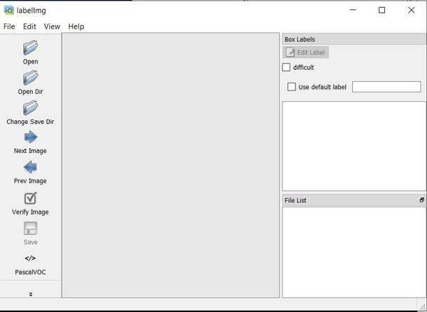
If you see this window, you have successfully installed LabelImg. Here is a tutorial on how to label your own images. Congratulations!
Recognize Objects Using Your WebCam
Approach
Note: This section gets really technical. If you know the basics of computer vision and deep learning, it will make sense. Otherwise, it will not. You can skip this section and head straight to the Implementation section if you are not interested in what is going on under the hood of the object recognition application we are developing.
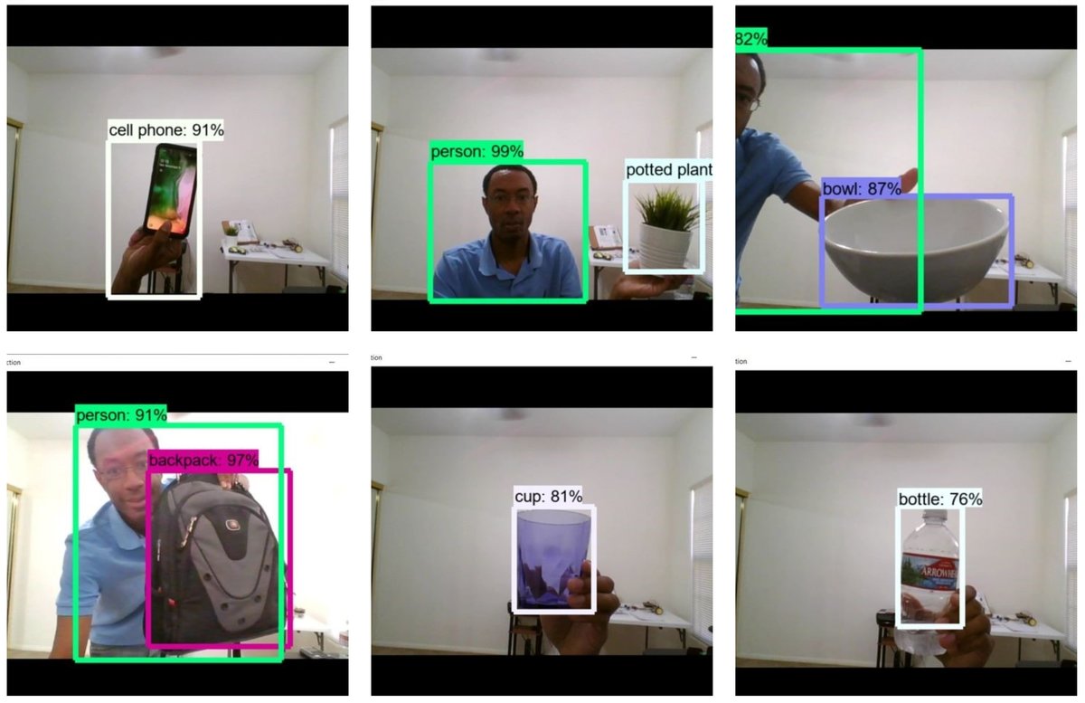
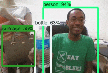
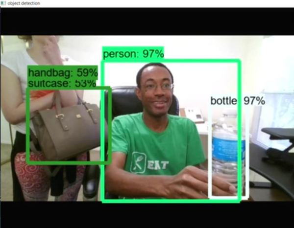
In this project, we use OpenCV and TensorFlow to create a system capable of automatically recognizing objects in a webcam. Each detected object is outlined with a bounding box labeled with the predicted object type as well as a detection score.
The detection score is the probability that a bounding box contains the object of a particular type (e.g. the confidence a model has that an object identified as a “backpack” is actually a backpack).
The particular SSD with Inception v2 model used in this project is the ssd_inception_v2_coco model. The ssd_inception_v2_coco model uses the Single Shot MultiBox Detector (SSD) for its architecture and the Inception v2 framework for feature extraction.
Single Shot MultiBox Detector (SSD)
Most state-of-the-art object detection methods involve the following stages:
- Hypothesize bounding boxes
- Resample pixels or features for each box
- Apply a classifier
The Single Shot MultiBox Detector (SSD) eliminates the multi-stage process above and performs all object detection computations using just a single deep neural network.
Inception v2
Most state-of-the-art object detection methods based on convolutional neural networks at the time of the invention of Inception v2 added increasingly more convolution layers or neurons per layer in order to achieve greater accuracy. The problem with this approach is that it is computationally expensive and prone to overfitting. The Inception v2 architecture (as well as the Inception v3 architecture) was proposed in order to address these shortcomings.
Rather than stacking multiple kernel filter sizes sequentially within a convolutional neural network, the approach of the inception-based model is to perform a convolution on an input with multiple kernels all operating at the same layer of the network. By factorizing convolutions and using aggressive regularization, the authors were able to improve computational efficiency. Inception v2 factorizes the traditional 7 x 7 convolution into 3 x 3 convolutions.
Szegedy, Vanhoucke, Ioffe, Shlens, & Wojna, (2015) conducted an empirically-based demonstration in their landmark Inception v2 paper, which showed that factorizing convolutions and using aggressive dimensionality reduction can substantially lower computational cost while maintaining accuracy.
Data Set
The ssd_inception_v2_coco model used in this project is pretrained on the Common Objects in Context (COCO) data set (COCO data set), a large-scale data set that contains 1.5 million object instances and more than 200,000 labeled images. The COCO data required 70,000 crowd worker hours to gather, annotate, and organize images of objects in natural environments.
Software Dependencies
The following libraries form the object recognition backbone of the application implemented in this project:
- OpenCV, a library of programming functions for computer vision.
- Pillow, a library for manipulating images.
- Numpy, a library for scientific computing.
- Matplotlib, a library for creating graphs and visualizations.
- TensorFlow Object Detection API, an open source framework developed by Google that enables the development, training, and deployment of pre-trained object detection models.
Implementation
Now to the fun part, we will now recognize objects using our computer webcam.
Copy the following program, and save it to your TensorFlow\models\research\object_detection directory as object_detection_test.py .
# Import all the key libraries
import numpy as np
import os
import six.moves.urllib as urllib
import sys
import tarfile
import tensorflow as tf
import zipfile
import cv2

from collections import defaultdict
from io import StringIO
from matplotlib import pyplot as plt
from PIL import Image
from utils import label_map_util
from utils import visualization_utils as vis_util

# Define the video stream
cap = cv2.VideoCapture(0)

# Which model are we downloading?
# The models are listed here: https://github.com/tensorflow/models/blob/master/research/object_detection/g3doc/detection_model_zoo.md
MODEL_NAME = 'ssd_inception_v2_coco_2018_01_28'
MODEL_FILE = MODEL_NAME + '.tar.gz'
DOWNLOAD_BASE = 'http://download.tensorflow.org/models/object_detection/'

# Path to the frozen detection graph.
# This is the actual model that is used for the object detection.
PATH_TO_CKPT = MODEL_NAME + '/frozen_inference_graph.pb'

# List of the strings that is used to add the correct label for each box.
PATH_TO_LABELS = os.path.join('data', 'mscoco_label_map.pbtxt')

# Number of classes to detect
NUM_CLASSES = 90

# Download Model
opener = urllib.request.URLopener()
opener.retrieve(DOWNLOAD_BASE + MODEL_FILE, MODEL_FILE)
tar_file = tarfile.open(MODEL_FILE)
for file in tar_file.getmembers():
    file_name = os.path.basename(file.name)
    if 'frozen_inference_graph.pb' in file_name:
        tar_file.extract(file, os.getcwd())

# Load a (frozen) Tensorflow model into memory.
detection_graph = tf.Graph()
with detection_graph.as_default():
    od_graph_def = tf.GraphDef()
    with tf.gfile.GFile(PATH_TO_CKPT, 'rb') as fid:
        serialized_graph = fid.read()
        od_graph_def.ParseFromString(serialized_graph)
        tf.import_graph_def(od_graph_def, name='')

# Loading label map
# Label maps map indices to category names, so that when our convolution network
# predicts `5`, we know that this corresponds to `airplane`.  Here we use internal
# utility functions, but anything that returns a dictionary mapping integers to
# appropriate string labels would be fine
label_map = label_map_util.load_labelmap(PATH_TO_LABELS)
categories = label_map_util.convert_label_map_to_categories(
    label_map, max_num_classes=NUM_CLASSES, use_display_name=True)
category_index = label_map_util.create_category_index(categories)


# Helper code
def load_image_into_numpy_array(image):
    (im_width, im_height) = image.size
    return np.array(image.getdata()).reshape(
        (im_height, im_width, 3)).astype(np.uint8)

# Detection
with detection_graph.as_default():
    with tf.Session(graph=detection_graph) as sess:
        while True:

            # Read frame from camera
            ret, image_np = cap.read()
            # Expand dimensions since the model expects images to have shape: [1, None, None, 3]
            image_np_expanded = np.expand_dims(image_np, axis=0)
            # Extract image tensor
            image_tensor = detection_graph.get_tensor_by_name('image_tensor:0')
            # Extract detection boxes
            boxes = detection_graph.get_tensor_by_name('detection_boxes:0')
            # Extract detection scores
            scores = detection_graph.get_tensor_by_name('detection_scores:0')
            # Extract detection classes
            classes = detection_graph.get_tensor_by_name('detection_classes:0')
            # Extract number of detectionsd
            num_detections = detection_graph.get_tensor_by_name(
                'num_detections:0')
            # Actual detection.
            (boxes, scores, classes, num_detections) = sess.run(
                [boxes, scores, classes, num_detections],
                feed_dict={image_tensor: image_np_expanded})
            # Visualization of the results of a detection.
            vis_util.visualize_boxes_and_labels_on_image_array(
                image_np,
                np.squeeze(boxes),
                np.squeeze(classes).astype(np.int32),
                np.squeeze(scores),
                category_index,
                use_normalized_coordinates=True,
                line_thickness=8)

            # Display output
            cv2.imshow('object detection', cv2.resize(image_np, (800, 600)))

            if cv2.waitKey(25) & 0xFF == ord('q'):
                cv2.destroyAllWindows()
                break


print("We are finished! That was fun!")
Open a new terminal window.
Activate the TensorFlow GPU virtual environment.
conda activate tensorflow_gpu
cd into your TensorFlow\models\research\object_detection directory.
At the time of this writing, we need to use Numpy version 1.16.4. Type the following command to see what version of Numpy you have on your system.
pip show numpy
If it is not 1.16.4, execute the following commands:
pip uninstall numpy
pip install numpy==1.16.4
Now run, your program:
python object_detection_test.py
In about 30 to 90 seconds, you should see your webcam power up and object recognition take action. That’s it! Congratulations for making it to the end of this tutorial!
Keep building!