In this post, I will explain how the Laplacian of Gaussian (LoG) filter works. Laplacian of Gaussian is a popular edge detection algorithm.
Edge detection is an important part of image processing and computer vision applications. It is used to detect objects, locate boundaries, and extract features. Edge detection is about identifying sudden, local changes in the intensity values of the pixels in an image.
How LoG Works
Edge detection algorithms like the Sobel Operator work on the first derivative of an image. In other words, if we have a graph of the intensity values for each pixel in an image, the Sobel Operator takes a look at where the slope of the graph of the intensity reaches a peak, and that peak is marked as an edge.
For our 10×1 pixel image, the blue curve below is a plot of the intensity values, and the orange curve is the plot of the first derivative of the blue curve. In layman’s terms, the orange curve is a plot of the slope.
The orange curve peaks in the middle, so we know that is
likely an edge. When we look at the original source image, we confirm that yes,
it is an edge.
One limitation with the approach above is that the first derivative of an image might be subject to a lot of noise. Local peaks in the slope of the intensity values might be due to shadows or tiny color changes that are not edges at all.
An alternative to using the first derivative of an image is to use the second derivative, which is the slope of the first derivative curve (i.e. that orange curve above). Such a curve looks something like this (see the gray curve below):
An edge occurs where the graph of the second derivative
crosses zero. This second derivative-based method is called the Laplacian
algorithm.
The Laplacian algorithm is also
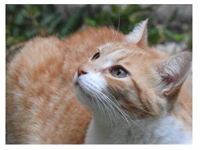
subject to noise. For example, consider a photo of a cat.
A cat hair or whisker might register as an edge because it is an area of a sharp change in intensity. However, it is not an edge. It is just noise. To solve this problem, a Gaussian smoothing filter is commonly applied to an image to reduce noise before the Laplacian is applied. This method is called the Laplacian of Gaussian (LoG).
We also set a threshold value to
distinguish noise from edges. If the second derivative magnitude at a pixel
exceeds this threshold, the pixel is part of an edge.
Mathematical Formulation of LoG
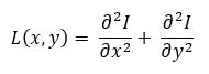
More formally, given a pixel (x, y), the Laplacian L(x,y) of an image with intensity values Ii can be written mathematically as follows:
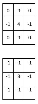
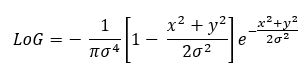
Just like in the case of the Sobel Operator, we cannot calculate the second derivative directly because pixels in an image are discrete. We need to approximate it using the convolution operator. The two most common kernels are:
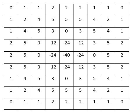
Calculating just the Laplacian will result in a lot of noise, so we need to convolve a Gaussian smoothing filter with the Laplacian filter to reduce noise prior to computing the second derivatives. The equation that combines both of these filters is called the Laplacian of Gaussian and is as follows:
The above equation is continuous,
so we need to discretize it so that we can use it on discrete pixels in an
image.
Here is an example of a LoG approximation
kernel where σ = 1.4. This is just an example of one convolution kernel
that can be used. There are others that would work as well.
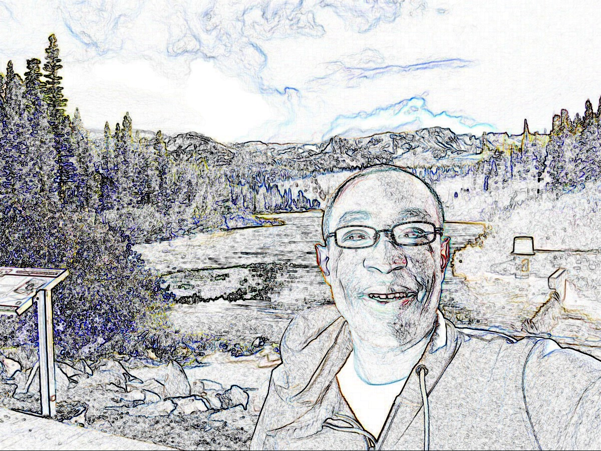
This LoG kernel is convolved with a grayscale input image to detect the zero crossings of the second derivative. We set a threshold for these zero crossings and retain only those zero crossings that exceed the threshold. Strong zero crossings are ones that have a big difference between the positive maximum and the negative minimum on either size of the zero crossing. Weak zero crossings are most likely noise, so they are ignored due to the thresholding we apply.
Laplacian of Gaussian Code
This tutorial has the Python code for the Laplacian of Gaussian.
In this post, I will explain how the Sobel Operator edge detection algorithm works.
The cover photo is what this photo looks like after the Sobel Operator has been applied.
In order to understand how the Sobel Operator detects edges, it is important to first understand how to model an edge. Let’s take a look at that now before we examine how the Sobel Operator works.
How to Model Edges Mathematically
Consider a grayscale image that is 10 x 1 pixels. Such an image would look something like the image below:
One can clearly see in the image that there is a sudden change in the intensity in the middle of the image. This sudden change is an edge.
Now, let us draw the corresponding intensity graph of each pixel, going from left to right. We will assume that black has an intensity of -1 (the lowest intensity), and white has an intensity of 1 (the highest intensity).
Mathematically, we can detect an abrupt change in the curve above by graphing the slope of the curve (i.e. taking the first derivative at each point along the curve).
The orange curve below is the graph of the slope at each point along the pixel intensity curve. Note how the curve reaches a maximum in the middle. This peak corresponds to an edge in the original image. It is an area where the intensity (brightness) of the image changes abruptly.
However, we have run into a problem here because I have drawn a continuous curve, but pixel intensity values are discrete. Therefore, in image processing, we cannot calculate the first derivatives of an image (known as “spatial derivatives”) directly using standard calculus methods; instead we have to estimate the derivative of the image using a mathematical operation known as convolution.
Professor Andrew Ng of Stanford University has a great video on how to perform the convolution operation given an input image:
I will explain the process below.
How to Perform the Convolution Operation Given an Image as Input
To do the convolution operation, we need to use a mathematical tool called a kernel (or filter). A kernel is just a fancy name for a small matrix.
Below is an example of a kernel.
This small matrix is 3×3 (3 rows and 3 columns). It happens to be the kernel
used in the Sobel algorithm to calculate estimates of the derivatives in the
vertical direction of an image. I will explain the Sobel algorithm later in
this section.
The middle cell in a kernel is
known as an anchor. In this case, the anchor is 0.
The Sobel Operator, a popular
edge detection algorithm, involves estimating the first derivative of an image
by doing a convolution between an image (i.e. the input) and two special
kernels, one to detect vertical edges and one to detect horizontal edges.
Let’s see how to estimate the first derivative of an image by doing an example convolution calculation…
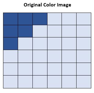
Suppose we have a 6×6 pixel color
image.
A color image has 3 channels (red, green and blue). To perform the convolution operation to detect edges, we only need one channel, so we first convert the image to grayscale. Converting the color image to grayscale is the first step of most of the edge detection algorithms, including the Sobel Operator algorithm.
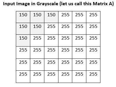
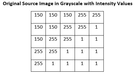
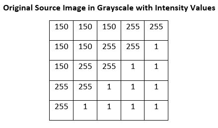
Here are what the intensity values might look like after the grayscale conversion.
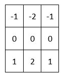
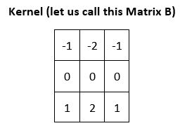
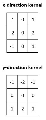
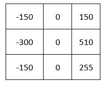
Now, consider the kernel below (this happens to be the Sobel Vertical Kernel used to detect vertical edges).
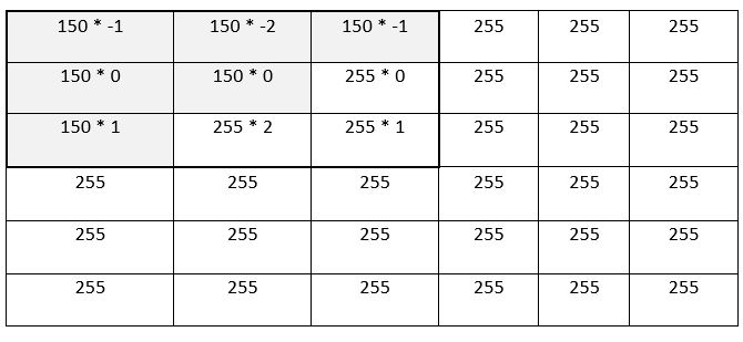
To convolve matrix A with matrix B, we first overlay Matrix B on top of the upper-left portion of Matrix A and then take the element-wise product:
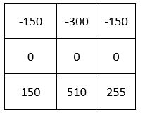
After completing the 9 multiplications, that upper-left portion becomes…
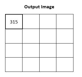
To complete the convolution operation, we add up all the numbers in the matrix above to get:
The output matrix for convolving matrix A with matrix B,
will be a 4×4 matrix. The value above, 315, becomes the first entry into this
output matrix. You can see that 315 is a relatively large number.
We keep shifting the 3×3 kernel over the image, pixel by pixel, until we have filled up the output matrix above. That is the convolution operation.
How the Sobel Operator Works
The Sobel Operator uses kernels and the convolution operation (described above) to detect edges in an image. The algorithm works with two kernels
A kernel to approximate intensity change in the x-direction (horizontal)
A kernel to approximate intensity change at a pixel in the y-direction (vertical).
In mathematical jargon, “approximating the intensity change” means approximating the gradient of the intensity values at a pixel. The gradient is the multivariable generalization of the derivative or slope mentioned earlier in this discussion.
Here are the two special kernels
used in the Sobel algorithm:
The two kernels above are convolved with each pixel in the original image to identify the regions where the change (gradient) is maximized in magnitude in the x and y directions.
Mathematical Formulation of the Sobel Operator
More formally,
Let gradient approximations in the x-direction be denoted as Gx
Let gradient approximations in the y-direction be denoted as Gy.
Suppose we have a source image Ii.
We want to calculate the magnitude of the gradient at a pixel (x, y), so we extract from image Ii a 3×3 matrix with pixel (x,y) as the center pixel (i.e. anchor).
The gradient approximations at
pixel (x,y) given a 3×3 portion of the source image Ii are calculated
as follows:
Gx = x-direction
kernel * (3×3 portion of image A with (x,y) as the center cell)
Gy = y-direction
kernel * (3×3 portion of image A with (x,y) as the center cell)
* above is not normal matrix
multiplication. * denotes the convolution operation I described earlier in this
discussion.
We then combine the values above
to calculate the magnitude of the gradient at pixel (x,y):
magnitude(G) =
square_root(Gx2 + Gy2)
The direction of the gradient Ɵ at pixel (x, y) is:
Ɵ =
atan(Gy / Gx)
where atan is the arctangent
operator.
So, in short, the algorithm goes
through each pixel in an image and defines 3×3 matrices that have that pixel as
the center cell (anchor pixel). Convolving these matrices with both the x and
y-direction kernels yields two values, gradient approximations in the x-direction
(Gx) and y-direction (Gy). We square both of these
values, add them, and then take the square root of the sum to calculate the
magnitude of the gradient at that pixel. Pixels that have gradients of large
magnitude are likely part of an edge in an image.
Example Calculation
Here is an example calculation showing
how to calculate the gradient approximation at a single pixel in the Sobel algorithm.
We have already converted the input image into grayscale:
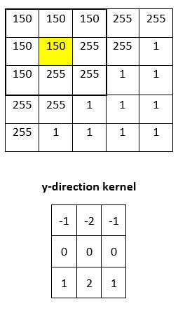
We start the calculation of the gradient in the y-direction (Gy) at the pixel in the second column and second row (marked in yellow).
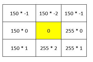
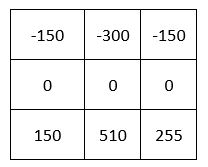
First, we convolve the selection in the original image with the y-direction kernel. The result is as follows:
Which becomes…
Then we add up all the numbers in the matrix above:
Gy for the
pixel in row 2, column 2 is 315.
We now do a similar calculation
to calculate Gx at that same pixel.The only thing that
changes is the kernel that we multiply our selection by.
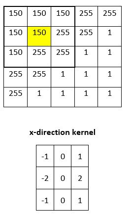
We start the calculation of the gradient in the x-direction (Gx) at the pixel in the second column and second row (marked in yellow).
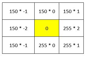
We convolve the selection in the original image with the x-direction kernel. The result is:
Which becomes…
Then we add up all the numbers in the matrix above:
Gx for the
pixel in row 2, column 2 is 315.
Thus, at the pixel at row 2,
column 2…
Gx = 315
Gy = 315
We then combine the values above
to calculate the magnitude of the gradient at pixel (x,y):
magnitude(G) =
square_root(Gx2 + Gy2)
magnitude(G) =
square_root(3152 + 3152)
magnitude(G) ≈ 445
This magnitude above is just our calculation for a single 3×3 region. We have to do the same thing for the other 3×3 regions in the image. And once we have done those calculations, we know that the pixels with the highest magnitude(G) are likely part of an edge.
This tutorial
on GitHub has a really nice animated demonstration of the Sobel Edge
Detection algorithm I explained above.
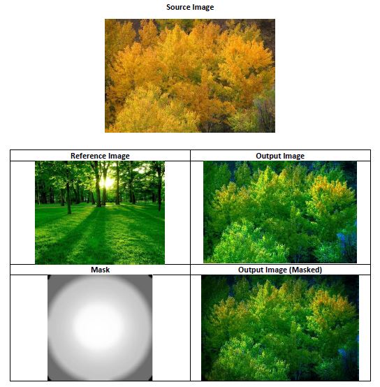
In this tutorial, you will learn how to do histogram matchingusing OpenCV. Histogram matching (also known as histogram specification), is the transformation of an image so that its histogram matches the histogram of an image of your choice (we’ll call this image of your choice the “reference image”).
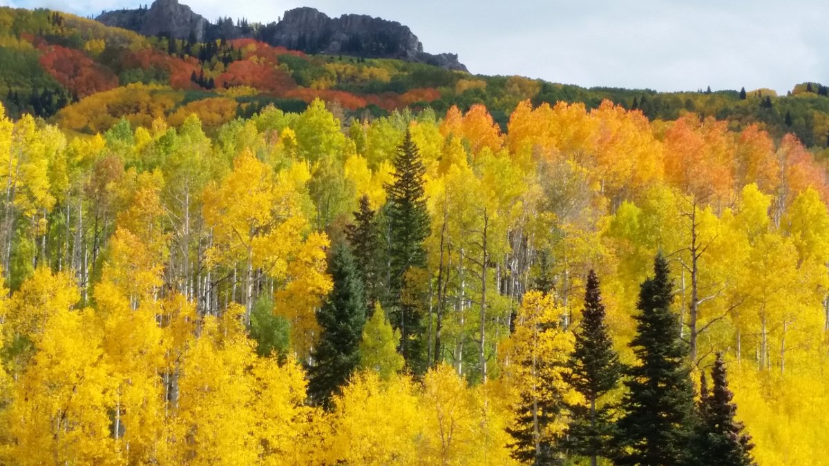
For example, consider this image below.
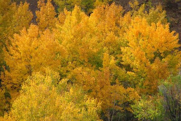
We want the image above to match the histogram of the reference image below.
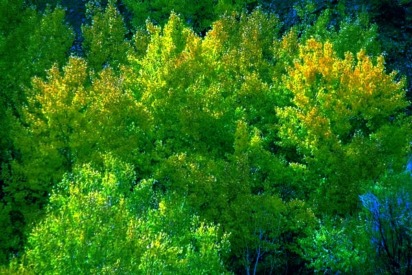
After performing histogram matching, the output image needs to look like this:
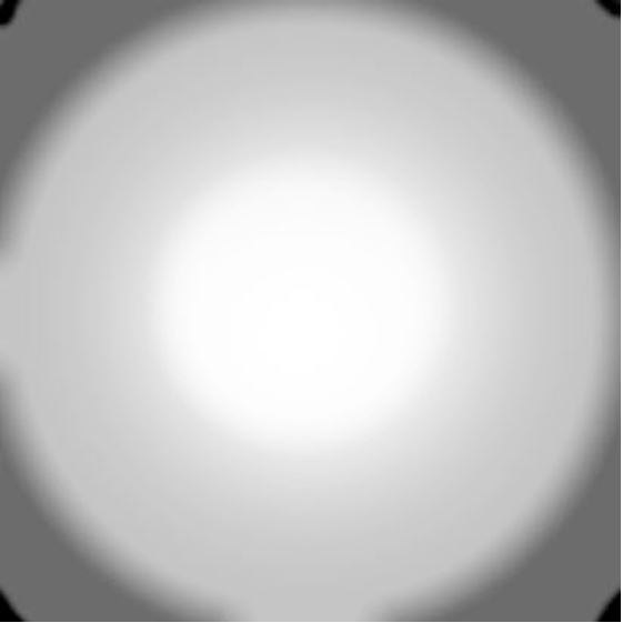
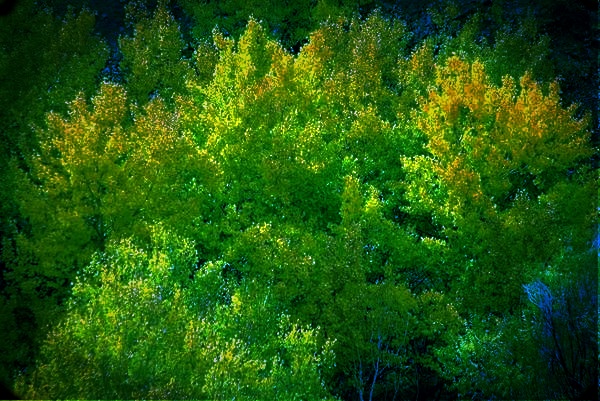
Then, to make things interesting, we want to use this mask to mask the output image.
Below is the source code for the program that makes everything happen. Make sure you copy and paste this code into a single Python file (mine is named histogram_matching.py). Then put that file, as well as your source, reference, and mask images all in the same directory (or folder) in your computer. Once you have done that, run the code using the following command (note: mask image is optional):
#!/usr/bin/env python

'''
Welcome to the Histogram Matching Program!

Given a source image and a reference image, this program
returns a modified version of the source image that matches
the histogram of the reference image.

Image Requirements:
  - Source image must be color.
  - Reference image must be color.
  - The sizes of the source image and reference image do not
    have to be the same.
  - The program supports an optional third image (mask) as
    an argument.
  - When the mask image is provided, it will be rescaled to
    be the same size as the source image, and the resulting
    matched image will be masked by the mask image.

Usage:
  python histogram_matching.py <source_image> <ref_image> [<mask_image>]
'''

# Python 2/3 compatibility
from __future__ import print_function

import cv2 # Import the OpenCV library
import numpy as np # Import Numpy library
import matplotlib.pyplot as plt # Import matplotlib functionality
import sys # Enables the passing of arguments

# Project: Histogram Matching Using OpenCV
# Author: Addison Sears-Collins
# Date created: 9/27/2019
# Python version: 3.7

# Define the file name of the images
SOURCE_IMAGE = "aspens_in_fall.jpg"
REFERENCE_IMAGE = "forest_resized.jpg"
MASK_IMAGE = "mask.jpg"
OUTPUT_IMAGE = "aspens_in_fall_forest_output"
OUTPUT_MASKED_IMAGE = "aspens_in_fall_forest_output_masked.jpg"

def calculate_cdf(histogram):
    """
    This method calculates the cumulative distribution function
    :param array histogram: The values of the histogram
    :return: normalized_cdf: The normalized cumulative distribution function
    :rtype: array
    """
    # Get the cumulative sum of the elements
    cdf = histogram.cumsum()

    # Normalize the cdf
    normalized_cdf = cdf / float(cdf.max())

    return normalized_cdf

def calculate_lookup(src_cdf, ref_cdf):
    """
    This method creates the lookup table
    :param array src_cdf: The cdf for the source image
    :param array ref_cdf: The cdf for the reference image
    :return: lookup_table: The lookup table
    :rtype: array
    """
    lookup_table = np.zeros(256)
    lookup_val = 0
    for src_pixel_val in range(len(src_cdf)):
        lookup_val
        for ref_pixel_val in range(len(ref_cdf)):
            if ref_cdf[ref_pixel_val] >= src_cdf[src_pixel_val]:
                lookup_val = ref_pixel_val
                break
        lookup_table[src_pixel_val] = lookup_val
    return lookup_table

def match_histograms(src_image, ref_image):
    """
    This method matches the source image histogram to the
    reference signal
    :param image src_image: The original source image
    :param image  ref_image: The reference image
    :return: image_after_matching
    :rtype: image (array)
    """
    # Split the images into the different color channels
    # b means blue, g means green and r means red
    src_b, src_g, src_r = cv2.split(src_image)
    ref_b, ref_g, ref_r = cv2.split(ref_image)

    # Compute the b, g, and r histograms separately
    # The flatten() Numpy method returns a copy of the array c
    # collapsed into one dimension.
    src_hist_blue, bin_0 = np.histogram(src_b.flatten(), 256, [0,256])
    src_hist_green, bin_1 = np.histogram(src_g.flatten(), 256, [0,256])
    src_hist_red, bin_2 = np.histogram(src_r.flatten(), 256, [0,256])
    ref_hist_blue, bin_3 = np.histogram(ref_b.flatten(), 256, [0,256])
    ref_hist_green, bin_4 = np.histogram(ref_g.flatten(), 256, [0,256])
    ref_hist_red, bin_5 = np.histogram(ref_r.flatten(), 256, [0,256])

    # Compute the normalized cdf for the source and reference image
    src_cdf_blue = calculate_cdf(src_hist_blue)
    src_cdf_green = calculate_cdf(src_hist_green)
    src_cdf_red = calculate_cdf(src_hist_red)
    ref_cdf_blue = calculate_cdf(ref_hist_blue)
    ref_cdf_green = calculate_cdf(ref_hist_green)
    ref_cdf_red = calculate_cdf(ref_hist_red)

    # Make a separate lookup table for each color
    blue_lookup_table = calculate_lookup(src_cdf_blue, ref_cdf_blue)
    green_lookup_table = calculate_lookup(src_cdf_green, ref_cdf_green)
    red_lookup_table = calculate_lookup(src_cdf_red, ref_cdf_red)

    # Use the lookup function to transform the colors of the original
    # source image
    blue_after_transform = cv2.LUT(src_b, blue_lookup_table)
    green_after_transform = cv2.LUT(src_g, green_lookup_table)
    red_after_transform = cv2.LUT(src_r, red_lookup_table)

    # Put the image back together
    image_after_matching = cv2.merge([
        blue_after_transform, green_after_transform, red_after_transform])
    image_after_matching = cv2.convertScaleAbs(image_after_matching)

    return image_after_matching

def mask_image(image, mask):
    """
    This method overlays a mask on top of an image
    :param image image: The color image that you want to mask
    :param image mask: The mask
    :return: masked_image
    :rtype: image (array)
    """

    # Split the colors into the different color channels
    blue_color, green_color, red_color = cv2.split(image)

    # Resize the mask to be the same size as the source image
    resized_mask = cv2.resize(
        mask, (image.shape[1], image.shape[0]), cv2.INTER_NEAREST)

    # Normalize the mask
    normalized_resized_mask = resized_mask / float(255)

    # Scale the color values
    blue_color = blue_color * normalized_resized_mask
    blue_color = blue_color.astype(int)
    green_color = green_color * normalized_resized_mask
    green_color = green_color.astype(int)
    red_color = red_color * normalized_resized_mask
    red_color = red_color.astype(int)

    # Put the image back together again
    merged_image = cv2.merge([blue_color, green_color, red_color])
    masked_image = cv2.convertScaleAbs(merged_image)
    return masked_image

def main():
    """
    Main method of the program.
    """
    start_the_program = input("Press ENTER to perform histogram matching...")

    # A flag to indicate if the mask image was provided or not by the user
    mask_provided = False

    # Pull system arguments
    try:
        image_src_name = sys.argv[1]
        image_ref_name = sys.argv[2]
    except:
        image_src_name = SOURCE_IMAGE
        image_ref_name = REFERENCE_IMAGE

    try:
        image_mask_name = sys.argv[3]
        mask_provided = True
    except:
        print("\nNote: A mask was not provided.\n")

    # Load the images and store them into a variable
    image_src = cv2.imread(cv2.samples.findFile(image_src_name))
    image_ref = cv2.imread(cv2.samples.findFile(image_ref_name))

    image_mask = None
    if mask_provided:
        image_mask = cv2.imread(cv2.samples.findFile(image_mask_name))

    # Check if the images loaded properly
    if image_src is None:
        print('Failed to load source image file:', image_src_name)
        sys.exit(1)
    elif image_ref is None:
        print('Failed to load reference image file:', image_ref_name)
        sys.exit(1)
    else:
        # Do nothing
        pass

    # Convert the image mask to grayscale
    if mask_provided:
        image_mask = cv2.cvtColor(image_mask, cv2.COLOR_BGR2GRAY)

    # Calculate the matched image
    output_image = match_histograms(image_src, image_ref)

    # Mask the matched image
    if mask_provided:
        output_masked = mask_image(output_image, image_mask)

    # Save the output images
    cv2.imwrite(OUTPUT_IMAGE, output_image)
    if mask_provided:
        cv2.imwrite(OUTPUT_MASKED_IMAGE, output_masked)

    ## Display images, used for debugging
    cv2.imshow('Source Image', image_src)
    cv2.imshow('Reference Image', image_ref)
    cv2.imshow('Output Image', output_image)
    if mask_provided:
        cv2.imshow('Mask', image_mask)
        cv2.imshow('Output Image (Masked)', output_masked)

    cv2.waitKey(0) # Wait for a keyboard event

if __name__ == '__main__':
    print(__doc__)
    main()
    cv2.destroyAllWindows()