In this post, I will explain the difference between histogram equalization and histogram matching. If you are in a hurry, here is the short answer: while the goal of histogram equalization is to produce an output image that has a flattened histogram, the goal of histogram matching is to take an input image and generate an output image that is based upon the shape of a specific (or reference) histogram.
Let’s take a look at the long answer by first examining the definition of a histogram (continued after the Table of Contents).
Table of Contents
- What is a Histogram?
- Histogram Equalization
- –How Histogram Equalization Works
- –Example of Histogram Equalization
- Histogram Matching
- –Example of Histogram Matching
What is a Histogram?
In image processing, a histogram shows the number of pixels (or voxels in the case of a 3D image) for each intensity value in a given image.
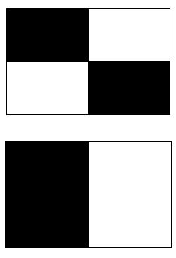
A histogram is a statistical representation of an image. It doesn’t show any information about where the pixels are located in the image. Therefore, two different images can have equivalent histograms. For example, the two images below are different but have identical histograms because both are 50% white (grayscale value of 255) and 50% black (grayscale value of 0).
Histogram Equalization
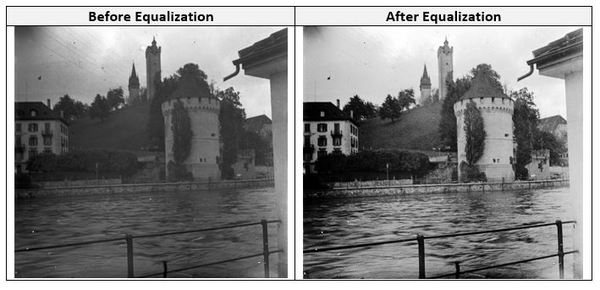
In histogram equalization (also known as histogram flattening), the goal is to improve contrast in images that might be either blurry or have a background and foreground that are either both bright or both dark. Histogram equalization helps sharpen an image.
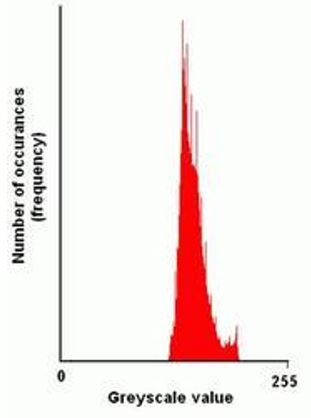
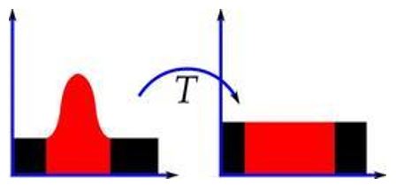
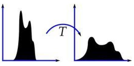
Low contrast images typically have histograms that are concentrated within a tight range of values. Histogram equalization can improve the contrast in these images by spreading out the histogram so that the intensity values are distributed uniformly over a larger intensity range. Ideally, the histogram of the output image will be perfectly flat.
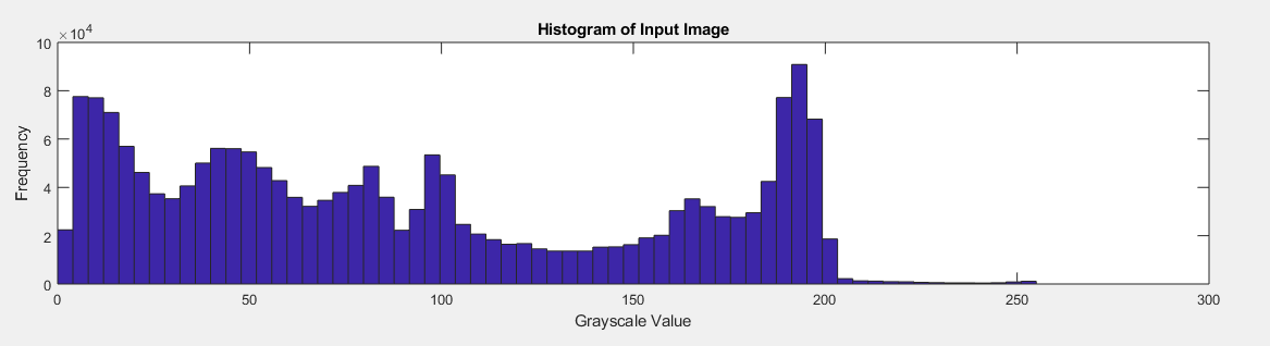
The two images below are two examples of what the histogram for an input image might look like before and after it goes through histogram equalization.
Histogram equalization is useful in a number of real-world use cases, such as x-rays, thermal imagery, and satellite photos.
Here is some Python code you can use to perform histogram equalization:
# Author: Addison Sears-Collins
# https://automaticaddison.com
# Description: Sharpen an image (i.e. increase contrast)
# using histogram equalization

import cv2 # Computer vision library
import numpy as np # Scientific computing library

# Read the image
img = cv2.imread('before.jpg',0)

# Perform histogram equalization
equ = cv2.equalizeHist(img)

# Stack images side-by-side
after = np.hstack((img,equ))

# Save the output image
cv2.imwrite('after.jpg',after)
Here is the input:
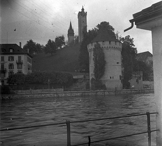
Here is the output generated by the program:
How Histogram Equalization Works
The process for histogram equalization is as follows:
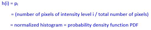
Step 1: Obtain the histogram.
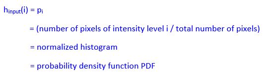
For example, if the image is grayscale with 256 distinct intensity levels i (where i = 0 [black], 1, 2, …. 253, 254, 255 [white]), the probability that a pixel chosen at random will have an intensity level i is as follows:
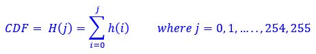
Step 2: Obtain the cumulative distribution function CDF.
The cumulative distribution function H(j) is defined as the probability H of a randomly selected pixel taking one of the intensity values from 0 through j (inclusive). Therefore, given our normalized histogram h(i) from above, we have the following formula:
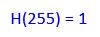
The sum of all the components in the normalized histogram is equal to 1. Therefore,
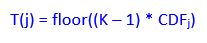
Step 3: Calculate the transformation T to map the old intensity values to new intensity values.
Let K represent the total number of possible intensity values (e.g. 256). j is the old intensity value, and T(j) is the new intensity value.
Step 4: Given the new mappings of intensity values, we can use a lookup table to transform each pixel in the input image to a new intensity.
The result of this transformation is a new histogram which corresponds to a new output image.
Special note on transformation functions:
The formula I used for histogram equalization is a common one, but other transformation functions are possible. Different transformation functions will yield different output histograms.
Example of Histogram Equalization
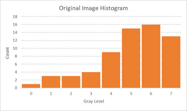
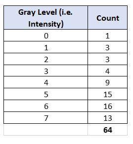
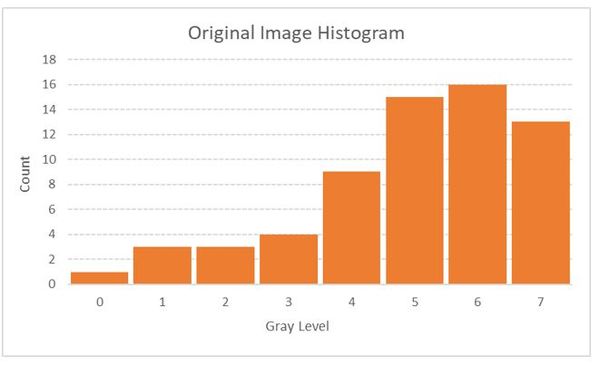
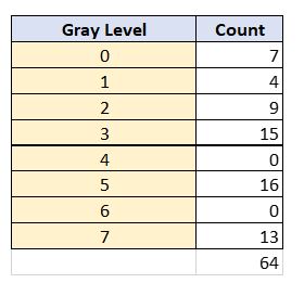
Let us suppose we have a 3-bit, 8 x 8 grayscale image. The grayscale range is 23 = 8 intensity values (i.e. gray levels) because the image is 3 bits. We label these intensity values 0 through 7. Below is the histogram of this image.
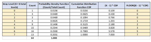
Now, we calculate the cumulative distribution function and perform the transformation.
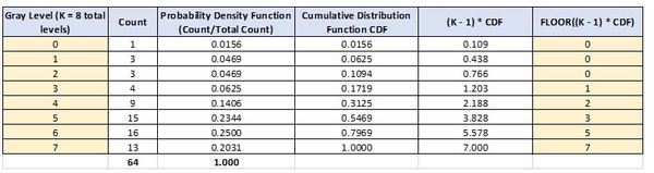
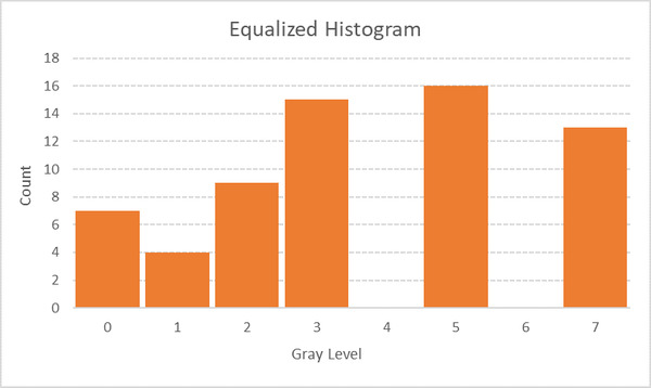
The two yellow columns above are our lookup table. We use these two columns to generate the output image. For example, we map all pixels that had a gray level of 3 to 1. We map all pixels that had a gray level of 6 to 5, etc. The resulting histogram looks like this:

Histogram Matching
While the goal of histogram equalization is to produce an output image that has a flattened histogram, the goal of histogram matching is to take an input image and generate an output image that is based upon the shape of a specific (or reference) histogram. Histogram matching is also known as histogram specification. You can consider histogram equalization as a special case of histogram matching in which we want to force an image to have a uniform histogram (rather than just any shape as is the case for histogram matching).
Let us suppose we have two images, an input image and a specified image. We want to use histogram matching to force the input image to have a histogram that is the shape of the histogram of the specified image. The first few steps are similar to histogram equalization, except we are performing histogram equalization on two images (original image and the specific image).
Step 1: Obtain the histogram for both the input image and the specified image (same method as in histogram equalization).
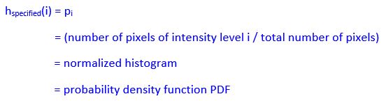
For example, if both images are grayscale with 256 distinct intensity levels i (where i = 0 [black], 1, 2, …. 253, 254, 255 [white]), the probability that a pixel chosen at random will have an intensity level i is as follows:
Step 2: Obtain the cumulative distribution function CDF for both the input image and the specified image (same method as in histogram equalization).
The cumulative distribution function H(j) is defined as the probability H of a randomly selected pixel taking one of the intensity values from 0 through j (inclusive). Therefore, given our normalized histograms h(i) from above, we have the following formula:

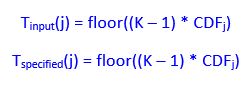
Step 3: Calculate the transformation T to map the old intensity values to new intensity values for both the input image and specified image (same method as in histogram equalization).
Let K represent the total number of possible intensity values (e.g. 256). j is the old intensity value, and T(j) is the new intensity value.
Step 4: Use the transformed intensity values for both the input image and specified image to map the intensity values of the input image to new values
We go through each available intensity value j one at a time, doing the following steps:
- See what the transformed intensity value is for the input image given the intensity value j. Let us call this Tinput(j).
- We then find the Tspecified(j) that is closest to Tinput(j) and make a note of what j is. For example, if j = 4:
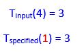
we map all intensity values of 4 in the input image to 1.
Here is another example. Let us suppose that:
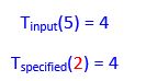
Therefore, we map all intensity values of 5 in the input image to 2.
After we have gone through all available intensity values and performed all the mappings, we have our output image which has a histogram that will approximately match the shape of the unequalized specified histogram.
Example of Histogram Matching
Let us take a look at an example. For convenience, I am reposting the unequalized and equalized histogram from the histogram equalization example.
Here is the histogram of the original image.

Now, we equalize the original input image to get the following table and histogram.
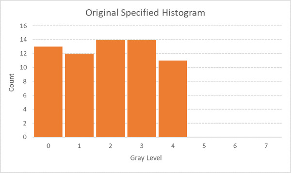
Now, let us suppose we have the following specified histogram. We want to get the original image to have a histogram that is shaped like the specified histogram.
We equalize the specified histogram, yielding the following table.
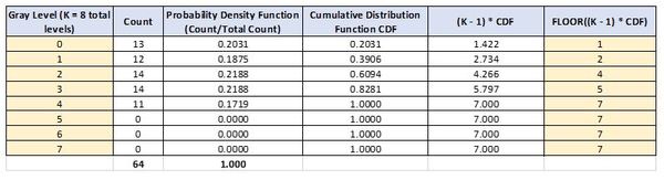
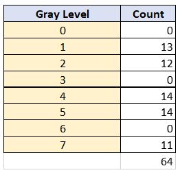
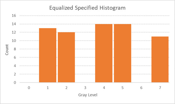
Using the two yellow columns above to map the old intensity values for the pixels to new intensity values, we get the following histogram after equalization:
Now, we need to use the transformed intensity values for both the input image and specified image to map the intensity values of the input image to new values. To do that, all we need are the FLOOR((K – 1) * CDF) values for both the original image and the specified image.
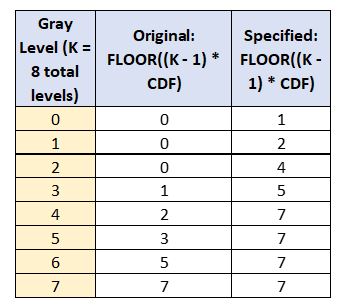
We go through each available intensity value j one at a time, doing the following steps:
- See what the transformed intensity value is for the input image given the intensity value j. Call this Tinput(j).
- We then find the Tspecified(j) that is closest to Tinput(j) and make a note of what j is.
For example, when the gray level is 4, the original image is 2. 2 in the specified image corresponds to a gray level of 1. Therefore, we map 4 to 1.
When the gray level is 5, the original image is 3. 3 in the specified image is closest to 2 (go to the next lowest level by convention) corresponds to a gray level of 1. Therefore, we map 5 to 1.
Here is the final mapping.
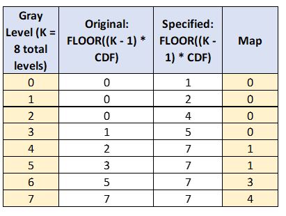
To finish the histogram matching process, we have to replace the values in the original image with the map values. The final matched histogram is shown below:
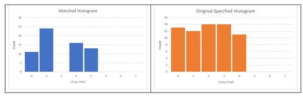
Therefore, the histogram matching process got us from the original image histogram below to that matched histogram above. Notice the matched histogram has a similar shape to the original specified histogram.