
In this post, I will explain how the Laplacian of Gaussian (LoG) filter works. Laplacian of Gaussian is a popular edge detection algorithm.
Edge detection is an important part of image processing and computer vision applications. It is used to detect objects, locate boundaries, and extract features. Edge detection is about identifying sudden, local changes in the intensity values of the pixels in an image.

How LoG Works
Edge detection algorithms like the Sobel Operator work on the first derivative of an image. In other words, if we have a graph of the intensity values for each pixel in an image, the Sobel Operator takes a look at where the slope of the graph of the intensity reaches a peak, and that peak is marked as an edge.
For our 10×1 pixel image, the blue curve below is a plot of the intensity values, and the orange curve is the plot of the first derivative of the blue curve. In layman’s terms, the orange curve is a plot of the slope.
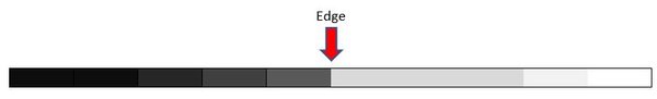
The orange curve peaks in the middle, so we know that is likely an edge. When we look at the original source image, we confirm that yes, it is an edge.
One limitation with the approach above is that the first derivative of an image might be subject to a lot of noise. Local peaks in the slope of the intensity values might be due to shadows or tiny color changes that are not edges at all.
An alternative to using the first derivative of an image is to use the second derivative, which is the slope of the first derivative curve (i.e. that orange curve above). Such a curve looks something like this (see the gray curve below):
An edge occurs where the graph of the second derivative crosses zero. This second derivative-based method is called the Laplacian algorithm.
The Laplacian algorithm is also subject to noise. For example, consider a photo of a cat.
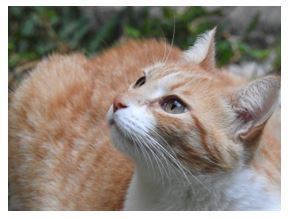
A cat hair or whisker might register as an edge because it is an area of a sharp change in intensity. However, it is not an edge. It is just noise. To solve this problem, a Gaussian smoothing filter is commonly applied to an image to reduce noise before the Laplacian is applied. This method is called the Laplacian of Gaussian (LoG).
We also set a threshold value to distinguish noise from edges. If the second derivative magnitude at a pixel exceeds this threshold, the pixel is part of an edge.
Mathematical Formulation of LoG
More formally, given a pixel (x, y), the Laplacian L(x,y) of an image with intensity values Ii can be written mathematically as follows:
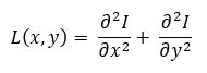
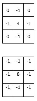
Just like in the case of the Sobel Operator, we cannot calculate the second derivative directly because pixels in an image are discrete. We need to approximate it using the convolution operator. The two most common kernels are:
Calculating just the Laplacian will result in a lot of noise, so we need to convolve a Gaussian smoothing filter with the Laplacian filter to reduce noise prior to computing the second derivatives. The equation that combines both of these filters is called the Laplacian of Gaussian and is as follows:
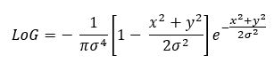
The above equation is continuous, so we need to discretize it so that we can use it on discrete pixels in an image.
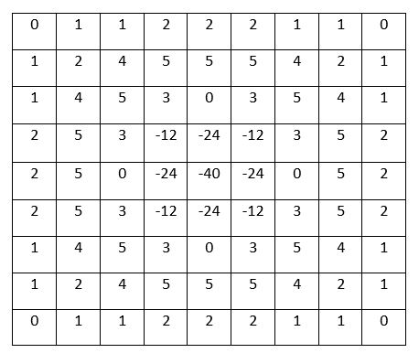
Here is an example of a LoG approximation kernel where σ = 1.4. This is just an example of one convolution kernel that can be used. There are others that would work as well.
This LoG kernel is convolved with a grayscale input image to detect the zero crossings of the second derivative. We set a threshold for these zero crossings and retain only those zero crossings that exceed the threshold. Strong zero crossings are ones that have a big difference between the positive maximum and the negative minimum on either size of the zero crossing. Weak zero crossings are most likely noise, so they are ignored due to the thresholding we apply.
Laplacian of Gaussian Code
This tutorial has the Python code for the Laplacian of Gaussian.