How to Determine the Orientation of an Object Using OpenCV

In this tutorial, we will build a program that can determine the orientation of an object (i.e. rotation angle in degrees) using the popular computer vision library OpenCV.

Real-World Applications

One of the most common real-world use cases of the program we will develop in this tutorial is when you want to develop a pick and place system for robotic arms. Determining the orientation of an object on a conveyor belt is key to determining the appropriate way to grasp the object, pick it up, and place it in another location.

Let’s get started!

Prerequisites

Installation and Setup

Before we get started, let’s make sure we have all the software packages installed. Check to see if you have OpenCV installed on your machine. If you are using Anaconda, you can type:

conda install -c conda-forge opencv

Alternatively, you can type:

pip install opencv-python

Install Numpy, the scientific computing library.

pip install numpy

Find an Image File

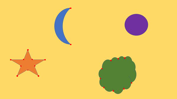
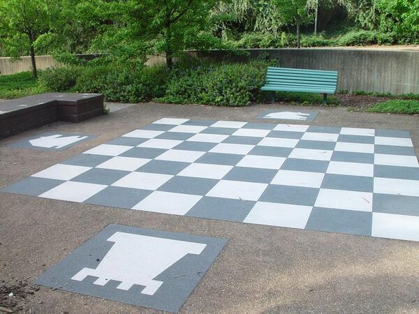
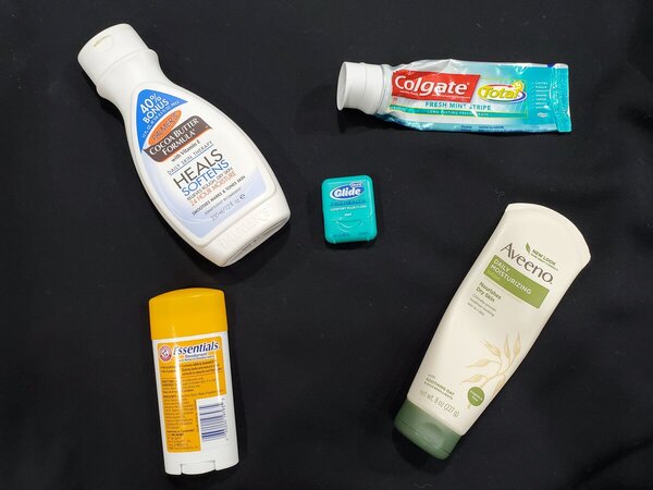
Find an image. My input image is 1200 pixels in width and 900 pixels in height. The filename of my input image is input_img.jpg.

input_img_600

Write the Code

Here is the code. It accepts an image named input_img.jpg and outputs an annotated image named output_img.jpg. Pieces of the code pull from the official OpenCV implementation.

import cv2 as cv
from math import atan2, cos, sin, sqrt, pi
import numpy as np

def drawAxis(img, p_, q_, color, scale):
  p = list(p_)
  q = list(q_)

  ## [visualization1]
  angle = atan2(p[1] - q[1], p[0] - q[0]) # angle in radians
  hypotenuse = sqrt((p[1] - q[1]) * (p[1] - q[1]) + (p[0] - q[0]) * (p[0] - q[0]))

  # Here we lengthen the arrow by a factor of scale
  q[0] = p[0] - scale * hypotenuse * cos(angle)
  q[1] = p[1] - scale * hypotenuse * sin(angle)
  cv.line(img, (int(p[0]), int(p[1])), (int(q[0]), int(q[1])), color, 3, cv.LINE_AA)

  # create the arrow hooks
  p[0] = q[0] + 9 * cos(angle + pi / 4)
  p[1] = q[1] + 9 * sin(angle + pi / 4)
  cv.line(img, (int(p[0]), int(p[1])), (int(q[0]), int(q[1])), color, 3, cv.LINE_AA)

  p[0] = q[0] + 9 * cos(angle - pi / 4)
  p[1] = q[1] + 9 * sin(angle - pi / 4)
  cv.line(img, (int(p[0]), int(p[1])), (int(q[0]), int(q[1])), color, 3, cv.LINE_AA)
  ## [visualization1]

def getOrientation(pts, img):
  ## [pca]
  # Construct a buffer used by the pca analysis
  sz = len(pts)
  data_pts = np.empty((sz, 2), dtype=np.float64)
  for i in range(data_pts.shape[0]):
    data_pts[i,0] = pts[i,0,0]
    data_pts[i,1] = pts[i,0,1]

  # Perform PCA analysis
  mean = np.empty((0))
  mean, eigenvectors, eigenvalues = cv.PCACompute2(data_pts, mean)

  # Store the center of the object
  cntr = (int(mean[0,0]), int(mean[0,1]))
  ## [pca]

  ## [visualization]
  # Draw the principal components
  cv.circle(img, cntr, 3, (255, 0, 255), 2)
  p1 = (cntr[0] + 0.02 * eigenvectors[0,0] * eigenvalues[0,0], cntr[1] + 0.02 * eigenvectors[0,1] * eigenvalues[0,0])
  p2 = (cntr[0] - 0.02 * eigenvectors[1,0] * eigenvalues[1,0], cntr[1] - 0.02 * eigenvectors[1,1] * eigenvalues[1,0])
  drawAxis(img, cntr, p1, (255, 255, 0), 1)
  drawAxis(img, cntr, p2, (0, 0, 255), 5)

  angle = atan2(eigenvectors[0,1], eigenvectors[0,0]) # orientation in radians
  ## [visualization]

  # Label with the rotation angle
  label = "  Rotation Angle: " + str(-int(np.rad2deg(angle)) - 90) + " degrees"
  textbox = cv.rectangle(img, (cntr[0], cntr[1]-25), (cntr[0] + 250, cntr[1] + 10), (255,255,255), -1)
  cv.putText(img, label, (cntr[0], cntr[1]), cv.FONT_HERSHEY_SIMPLEX, 0.5, (0,0,0), 1, cv.LINE_AA)

  return angle

# Load the image
img = cv.imread("input_img.jpg")

# Was the image there?
if img is None:
  print("Error: File not found")
  exit(0)

cv.imshow('Input Image', img)

# Convert image to grayscale
gray = cv.cvtColor(img, cv.COLOR_BGR2GRAY)

# Convert image to binary
_, bw = cv.threshold(gray, 50, 255, cv.THRESH_BINARY | cv.THRESH_OTSU)

# Find all the contours in the thresholded image
contours, _ = cv.findContours(bw, cv.RETR_LIST, cv.CHAIN_APPROX_NONE)

for i, c in enumerate(contours):

  # Calculate the area of each contour
  area = cv.contourArea(c)

  # Ignore contours that are too small or too large
  if area < 3700 or 100000 < area:
    continue

  # Draw each contour only for visualisation purposes
  cv.drawContours(img, contours, i, (0, 0, 255), 2)

  # Find the orientation of each shape
  getOrientation(c, img)

cv.imshow('Output Image', img)
cv.waitKey(0)
cv.destroyAllWindows()
 
# Save the output image to the current directory
cv.imwrite("output_img.jpg", img)
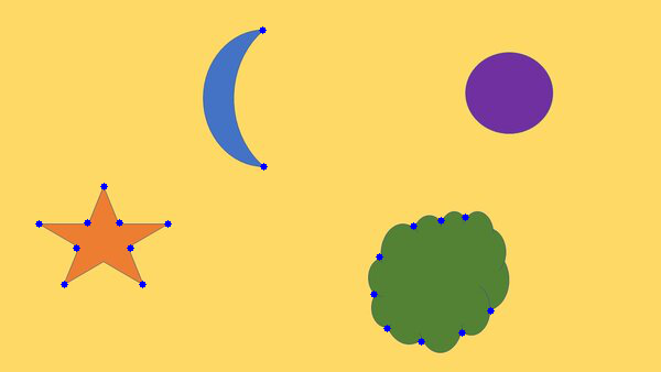
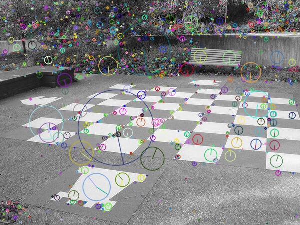
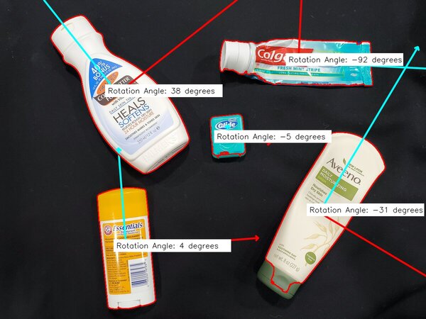
Output Image

Here is the result:

output_img_600-1

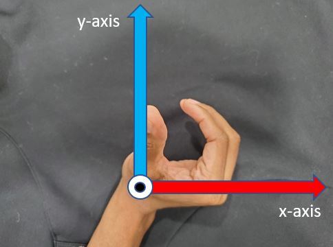
Understanding the Rotation Axes

The positive x-axis of each object is the red line. The positive y-axis of each object is the blue line

The global positive x-axis goes from left to right horizontally across the image. The global positive z-axis points out of this page. The global positive y-axis points from the bottom of the image to the top of the image vertically.

Using the right-hand rule to measure rotation, you stick your four fingers out straight (index finger to pinky finger) in the direction of the global positive x-axis.

right-hand-ruleJPG

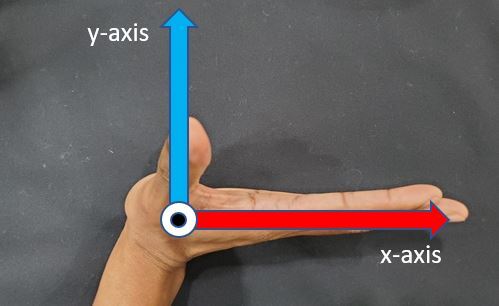
You then rotate your four fingers 90 degrees counterclockwise. Your fingertips point towards the positive y-axis, and your thumb points out of this page towards the positive z-axis.

right-hand-rule-curlJPG

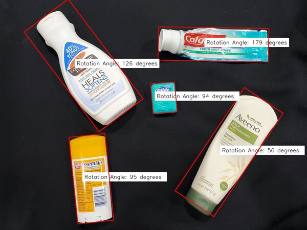
Calculate an Orientation Between 0 and 180 Degrees

If we want to calculate the orientation of an object and make sure that the result is always between 0 and 180 degrees, we can use this code:

# This programs calculates the orientation of an object.
# The input is an image, and the output is an annotated image
# with the angle of otientation for each object (0 to 180 degrees)

import cv2 as cv
from math import atan2, cos, sin, sqrt, pi
import numpy as np

# Load the image
img = cv.imread("input_img.jpg")

# Was the image there?
if img is None:
  print("Error: File not found")
  exit(0)

cv.imshow('Input Image', img)

# Convert image to grayscale
gray = cv.cvtColor(img, cv.COLOR_BGR2GRAY)

# Convert image to binary
_, bw = cv.threshold(gray, 50, 255, cv.THRESH_BINARY | cv.THRESH_OTSU)

# Find all the contours in the thresholded image
contours, _ = cv.findContours(bw, cv.RETR_LIST, cv.CHAIN_APPROX_NONE)

for i, c in enumerate(contours):

  # Calculate the area of each contour
  area = cv.contourArea(c)

  # Ignore contours that are too small or too large
  if area < 3700 or 100000 < area:
    continue

  # cv.minAreaRect returns:
  # (center(x, y), (width, height), angle of rotation) = cv2.minAreaRect(c)
  rect = cv.minAreaRect(c)
  box = cv.boxPoints(rect)
  box = np.int0(box)

  # Retrieve the key parameters of the rotated bounding box
  center = (int(rect[0][0]),int(rect[0][1])) 
  width = int(rect[1][0])
  height = int(rect[1][1])
  angle = int(rect[2])

  	
  if width < height:
    angle = 90 - angle
  else:
    angle = -angle
		
  label = "  Rotation Angle: " + str(angle) + " degrees"
  textbox = cv.rectangle(img, (center[0]-35, center[1]-25), 
    (center[0] + 295, center[1] + 10), (255,255,255), -1)
  cv.putText(img, label, (center[0]-50, center[1]), 
    cv.FONT_HERSHEY_SIMPLEX, 0.7, (0,0,0), 1, cv.LINE_AA)
  cv.drawContours(img,[box],0,(0,0,255),2)

cv.imshow('Output Image', img)
cv.waitKey(0)
cv.destroyAllWindows()
 
# Save the output image to the current directory
cv.imwrite("min_area_rec_output.jpg", img)

Here is the output:

min_area_rec_output

That’s it. Keep building!

Human Pose Estimation Using Deep Learning in OpenCV

In this tutorial, we will implement human pose estimation. Pose estimation means estimating the position and orientation of objects (in this case humans) relative to the camera. By the end of this tutorial, you will be able to generate the following output:

human_pose_gif-1

Real-World Applications

Human pose estimation has a number of real-world applications: 

Let’s get started!

Prerequisites

Installation and Setup

We need to make sure we have all the software packages installed. Check to see if you have OpenCV installed on your machine. If you are using Anaconda, you can type:

conda install -c conda-forge opencv

Alternatively, you can type:

pip install opencv-python

Make sure you have NumPy installed, a scientific computing library for Python.

If you’re using Anaconda, you can type:

conda install numpy

Alternatively, you can type:

pip install numpy

Find Some Videos

The first thing we need to do is find some videos to serve as our test cases.

We want to download videos that contain humans. The video files should be in mp4 format and 1920 x 1080 in dimensions.

I found some good candidates on Pixabay.com and Dreamstime.com

Take your videos and put them inside a directory on your computer.

Download the Protobuf File

Inside the same directory as your videos, download the protobuf file on this page. It is named graph_opt.pb. This file contains the weights of the neural network. The neural network is what we will use to determine the human’s position and orientation (i.e. pose).

Brief Description of OpenPose

We will use the OpenPose application along with OpenCV to do what we need to do in this project. OpenPose is an open source real-time 2D pose estimation application for people in video and images. It was developed by students and faculty members at Carnegie Mellon University. 

You can learn the theory and details of how OpenPose works in this paper and at GeeksforGeeks.

Write the Code

Here is the code. Make sure you put the code in the same directory on your computer where you put the other files.

The only lines you need to change are:

  • Line 14 (name of the input file in mp4 format)
  • Line 15 (input file size)
  • Line 18 (output file name)
# Project: Human Pose Estimation Using Deep Learning in OpenCV
# Author: Addison Sears-Collins
# Date created: February 25, 2021
# Description: A program that takes a video with a human as input and outputs
# an annotated version of the video with the human's position and orientation..

# Reference: https://github.com/quanhua92/human-pose-estimation-opencv

# Import the important libraries
import cv2 as cv # Computer vision library
import numpy as np # Scientific computing library

# Make sure the video file is in the same directory as your code
filename = 'dancing32.mp4'
file_size = (1920,1080) # Assumes 1920x1080 mp4 as the input video file

# We want to save the output to a video file
output_filename = 'dancing32_output.mp4'
output_frames_per_second = 20.0 

BODY_PARTS = { "Nose": 0, "Neck": 1, "RShoulder": 2, "RElbow": 3, "RWrist": 4,
               "LShoulder": 5, "LElbow": 6, "LWrist": 7, "RHip": 8, "RKnee": 9,
               "RAnkle": 10, "LHip": 11, "LKnee": 12, "LAnkle": 13, "REye": 14,
               "LEye": 15, "REar": 16, "LEar": 17, "Background": 18 }

POSE_PAIRS = [ ["Neck", "RShoulder"], ["Neck", "LShoulder"], ["RShoulder", "RElbow"],
               ["RElbow", "RWrist"], ["LShoulder", "LElbow"], ["LElbow", "LWrist"],
               ["Neck", "RHip"], ["RHip", "RKnee"], ["RKnee", "RAnkle"], ["Neck", "LHip"],
               ["LHip", "LKnee"], ["LKnee", "LAnkle"], ["Neck", "Nose"], ["Nose", "REye"],
               ["REye", "REar"], ["Nose", "LEye"], ["LEye", "LEar"] ]

# Width and height of training set
inWidth = 368
inHeight = 368

net = cv.dnn.readNetFromTensorflow("graph_opt.pb")

cap = cv.VideoCapture(filename)

# Create a VideoWriter object so we can save the video output
fourcc = cv.VideoWriter_fourcc(*'mp4v')
result = cv.VideoWriter(output_filename,  
                         fourcc, 
                         output_frames_per_second, 
                         file_size) 
# Process the video
while cap.isOpened():
    hasFrame, frame = cap.read()
    if not hasFrame:
        cv.waitKey()
        break

    frameWidth = frame.shape[1]
    frameHeight = frame.shape[0]
    
    net.setInput(cv.dnn.blobFromImage(frame, 1.0, (inWidth, inHeight), (127.5, 127.5, 127.5), swapRB=True, crop=False))
    out = net.forward()
    out = out[:, :19, :, :]  # MobileNet output [1, 57, -1, -1], we only need the first 19 elements

    assert(len(BODY_PARTS) == out.shape[1])

    points = []
    for i in range(len(BODY_PARTS)):
        # Slice heatmap of corresponging body's part.
        heatMap = out[0, i, :, :]

        # Originally, we try to find all the local maximums. To simplify a sample
        # we just find a global one. However only a single pose at the same time
        # could be detected this way.
        _, conf, _, point = cv.minMaxLoc(heatMap)
        x = (frameWidth * point[0]) / out.shape[3]
        y = (frameHeight * point[1]) / out.shape[2]
        # Add a point if it's confidence is higher than threshold.
        # Feel free to adjust this confidence value.  
        points.append((int(x), int(y)) if conf > 0.2 else None)

    for pair in POSE_PAIRS:
        partFrom = pair[0]
        partTo = pair[1]
        assert(partFrom in BODY_PARTS)
        assert(partTo in BODY_PARTS)

        idFrom = BODY_PARTS[partFrom]
        idTo = BODY_PARTS[partTo]

        if points[idFrom] and points[idTo]:
            cv.line(frame, points[idFrom], points[idTo], (0, 255, 0), 3)
            cv.ellipse(frame, points[idFrom], (3, 3), 0, 0, 360, (255, 0, 0), cv.FILLED)
            cv.ellipse(frame, points[idTo], (3, 3), 0, 0, 360, (255, 0, 0), cv.FILLED)

    t, _ = net.getPerfProfile()
    freq = cv.getTickFrequency() / 1000
    cv.putText(frame, '%.2fms' % (t / freq), (10, 20), cv.FONT_HERSHEY_SIMPLEX, 0.5, (0, 0, 0))

    # Write the frame to the output video file
    result.write(frame)
		
# Stop when the video is finished
cap.release()
	
# Release the video recording
result.release()

Run the Code

To run the code, type:

python openpose.py

Video Output

Here is the output I got:

Further Work

If you would like to do a deep dive into pose estimation, check out the official GitHub for the OpenPose project here.

That’s it. Keep building!

Image Feature Detection, Description, and Matching in OpenCV

In this tutorial, we will implement various image feature detection (a.k.a. feature extraction) and description algorithms using OpenCV, the computer vision library for Python. I’ll explain what a feature is later in this post.

We will also look at an example of how to match features between two images. This process is called feature matching.

Real-World Applications

  • Object Detection
  • Object Tracking
  • Object Classification

Let’s get started!

Prerequisites

What is a Feature?

Do you remember when you were a kid, and you played with puzzles? The objective was to put the puzzle pieces together. When the puzzle was all assembled, you would be able to see the big picture, which was usually some person, place, thing, or combination of all three.

jigsaw_puzzle_piece_grandmother

What enabled you to successfully complete the puzzle? Each puzzle piece contained some clues…perhaps an edge, a corner, a particular color pattern, etc. You used these clues to assemble the puzzle.

The “clues” in the example I gave above are image features. A feature in computer vision is a region of interest in an image that is unique and easy to recognize. Features include things like, points, edges, blobs, and corners.

For example, suppose you saw this feature?

Capture

You see some shaped, edges, and corners. These features are clues to what this object might be.

Now, let’s say we also have this feature.

2

Can you recognize what this object is?

Many Americans and people who have traveled to New York City would guess that this is the Statue of Liberty. And in fact, it is.

3_statue_of_liberty

With just two features, you were able to identify this object. Computers follow a similar process when you run a feature detection algorithm to perform object recognition.

The Python computer vision library OpenCV has a number of algorithms to detect features in an image. We will explore these algorithms in this tutorial.

Installation and Setup

Before we get started, let’s make sure we have all the software packages installed. Check to see if you have OpenCV installed on your machine. If you are using Anaconda, you can type:

conda install -c conda-forge opencv

Alternatively, you can type:

pip install opencv-python

Install Numpy, the scientific computing library.

pip install numpy

Install Matplotlib, the plotting library.

pip install matplotlib

Find an Image File

Find an image of any size. Here is mine:

random-shapes-small

Difference Between a Feature Detector and a Feature Descriptor

Before we get started developing our program, let’s take a look at some definitions. 

The algorithms for features fall into two categories: feature detectors and feature descriptors. 

A feature detector finds regions of interest in an image. The input into a feature detector is an image, and the output are pixel coordinates of the significant areas in the image.

A feature descriptor encodes that feature into a numerical “fingerprint”. Feature description makes a feature uniquely identifiable from other features in the image. 

We can then use the numerical fingerprint to identify the feature even if the image undergoes some type of distortion.

Feature Detection Algorithms

Harris Corner Detection

A corner is an area of an image that has a large variation in pixel color intensity values in all directions. One popular algorithm for detecting corners in an image is called the Harris Corner Detector.

Here is some basic code for the Harris Corner Detector. I named my file harris_corner_detector.py.

# Code Source: https://opencv-python-tutroals.readthedocs.io/en/latest/py_tutorials/py_feature2d/py_features_harris/py_features_harris.html

import cv2
import numpy as np

filename = 'random-shapes-small.jpg'
img = cv2.imread(filename)
gray = cv2.cvtColor(img,cv2.COLOR_BGR2GRAY)

gray = np.float32(gray)
dst = cv2.cornerHarris(gray,2,3,0.04)

#result is dilated for marking the corners, not important
dst = cv2.dilate(dst,None)

# Threshold for an optimal value, it may vary depending on the image.
img[dst>0.01*dst.max()]=[0,0,255]

cv2.imshow('dst',img)
if cv2.waitKey(0) & 0xff == 27:
    cv2.destroyAllWindows()

Here is my image before:

random-shapes-small-1

Here is my image after:

1-harris-corner-detection

For a more detailed example, check out my post “Detect the Corners of Objects Using Harris Corner Detector.”

Shi-Tomasi Corner Detector and Good Features to Track

Another corner detection algorithm is called Shi-Tomasi. Let’s run this algorithm on the same image and see what we get. Here is the code. I named the file shi_tomasi_corner_detect.py.

# Code Source: https://opencv-python-tutroals.readthedocs.io/en/latest/py_tutorials/py_feature2d/py_shi_tomasi/py_shi_tomasi.html

import numpy as np
import cv2
from matplotlib import pyplot as plt

img = cv2.imread('random-shapes-small.jpg')
gray = cv2.cvtColor(img,cv2.COLOR_BGR2GRAY)

# Find the top 20 corners
corners = cv2.goodFeaturesToTrack(gray,20,0.01,10)
corners = np.int0(corners)

for i in corners:
    x,y = i.ravel()
    cv2.circle(img,(x,y),3,255,-1)

cv2.imshow('Shi-Tomasi', img)
cv2.waitKey(0)
cv2.destroyAllWindows()

Here is the image after running the program:

2-shi-tomasi

Scale-Invariant Feature Transform (SIFT)

When we rotate an image or change its size, how can we make sure the features don’t change? The methods I’ve used above aren’t good at handling this scenario.

For example, consider these three images below of the Statue of Liberty in New York City. You know that this is the Statue of Liberty regardless of changes in the angle, color, or rotation of the statue in the photo. However, computers have a tough time with this task.

3_statue_of_liberty-1
4_statue_of_liberty
5_statue_of_liberty

OpenCV has an algorithm called SIFT that is able to detect features in an image regardless of changes to its size or orientation. This property of SIFT gives it an advantage over other feature detection algorithms which fail when you make transformations to an image.

Here is an example of code that uses SIFT:

# Code source: https://docs.opencv.org/master/da/df5/tutorial_py_sift_intro.html
import numpy as np
import cv2 as cv

# Read the image
img = cv.imread('chessboard.jpg')

# Convert to grayscale
gray = cv.cvtColor(img,cv.COLOR_BGR2GRAY)

# Find the features (i.e. keypoints) and feature descriptors in the image
sift = cv.SIFT_create()
kp, des = sift.detectAndCompute(gray,None)

# Draw circles to indicate the location of features and the feature's orientation
img=cv.drawKeypoints(gray,kp,img,flags=cv.DRAW_MATCHES_FLAGS_DRAW_RICH_KEYPOINTS)

# Save the image
cv.imwrite('sift_with_features_chessboard.jpg',img)

Here is the before:

chessboard

Here is the after. Each of those circles indicates the size of that feature. The line inside the circle indicates the orientation of the feature:

sift_with_features_chessboard

Speeded-up robust features (SURF)

SURF is a faster version of SIFT. It is another way to find features in an image.

Here is the code:

# Code Source: https://docs.opencv.org/master/df/dd2/tutorial_py_surf_intro.html

import numpy as np
import cv2 as cv

# Read the image
img = cv.imread('chessboard.jpg')

# Find the features (i.e. keypoints) and feature descriptors in the image
surf = cv.xfeatures2d.SURF_create(400)
kp, des = sift.detectAndCompute(img,None)

# Draw circles to indicate the location of features and the feature's orientation
img=cv.drawKeypoints(gray,kp,img,flags=cv.DRAW_MATCHES_FLAGS_DRAW_RICH_KEYPOINTS)

# Save the image
cv.imwrite('surf_with_features_chessboard.jpg',img)

Features from Accelerated Segment Test (FAST)

A lot of the feature detection algorithms we have looked at so far work well in different applications. However, they aren’t fast enough for some robotics use cases (e.g. SLAM). 

The FAST algorithm, implemented here, is a really fast algorithm for detecting corners in an image.

Blob Detectors With LoG, DoG, and DoH

A blob is another type of feature in an image. A blob is a region in an image with similar pixel intensity values. Another definition you will hear is that a blob is a light on dark or a dark on light area of an image.

Three popular blob detection algorithms are Laplacian of Gaussian (LoG), Difference of Gaussian (DoG), and Determinant of Hessian (DoH). 
Basic implementations of these blob detectors are at this page on the scikit-image website. Scikit-image is an image processing library for Python.

Feature Descriptor Algorithms

Histogram of Oriented Gradients

The HoG algorithm breaks an image down into small sections and calculates the gradient and orientation in each section. This information is then gathered into bins to compute histograms. These histograms give an image numerical “fingerprints” that make it uniquely identifiable.

A basic implementation of HoG is at this page.

Binary Robust Independent Elementary Features (BRIEF)

BRIEF is a fast, efficient alternative to SIFT. A sample implementation of BRIEF is here at the OpenCV website.

Oriented FAST and Rotated BRIEF (ORB)

SIFT was patented for many years, and SURF is still a patented algorithm. ORB was created in 2011 as a free alternative to these algorithms. It combines the FAST and BRIEF algorithms. You can find a basic example of ORB at the OpenCV website.

Feature Matching Example

You can use ORB to locate features in an image and then match them with features in another image.

For example, consider this Whole Foods logo. This logo will be our training image

training_image

I want to locate this Whole Foods logo inside this image below. This image below is our query image.

query_image

Here is the code you need to run. My file is called feature_matching_orb.py.

import numpy as np 
import cv2 
from matplotlib import pyplot as plt
	
# Read the training and query images
query_img = cv2.imread('query_image.jpg') 
train_img = cv2.imread('training_image.jpg') 

# Convert the images to grayscale 
query_img_gray = cv2.cvtColor(query_img,cv2.COLOR_BGR2GRAY) 
train_img_gray = cv2.cvtColor(train_img, cv2.COLOR_BGR2GRAY) 

# Initialize the ORB detector algorithm 
orb = cv2.ORB_create() 

# Detect keypoints (features) cand calculate the descriptors
query_keypoints, query_descriptors = orb.detectAndCompute(query_img_gray,None) 
train_keypoints, train_descriptors = orb.detectAndCompute(train_img_gray,None) 

# Match the keypoints
matcher = cv2.BFMatcher() 
matches = matcher.match(query_descriptors,train_descriptors) 

# Draw the keypoint matches on the output image
output_img = cv2.drawMatches(query_img, query_keypoints, 
train_img, train_keypoints, matches[:20],None) 

output_img = cv2.resize(output_img, (1200,650)) 

# Save the final image 
cv2.imwrite("feature_matching_result.jpg", output_img) 

# Close OpenCV upon keypress
cv2.waitKey(0)
cv2.destroyAllWindows()

Here is the result:

feature_matching_result_small

If you want to dive deeper into feature matching algorithms (Homography, RANSAC, Brute-Force Matcher, FLANN, etc.), check out the official tutorials on the OpenCV website. This page and this page have some basic examples.

That’s it. Keep building!