In this tutorial, we will implement various image feature detection (a.k.a. feature extraction) and description algorithms using OpenCV, the computer vision library for Python. I’ll explain what a feature is later in this post.
We will also look at an example of how to match features between two images. This process is called feature matching.
Real-World Applications
- Object Detection
- Object Tracking
- Object Classification
Let’s get started!
Prerequisites
What is a Feature?
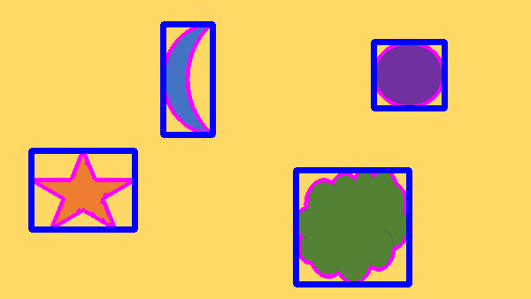
Do you remember when you were a kid, and you played with puzzles? The objective was to put the puzzle pieces together. When the puzzle was all assembled, you would be able to see the big picture, which was usually some person, place, thing, or combination of all three.
What enabled you to successfully complete the puzzle? Each puzzle piece contained some clues…perhaps an edge, a corner, a particular color pattern, etc. You used these clues to assemble the puzzle.
The “clues” in the example I gave above are image features. A feature in computer vision is a region of interest in an image that is unique and easy to recognize. Features include things like, points, edges, blobs, and corners.
For example, suppose you saw this feature?

You see some shaped, edges, and corners. These features are clues to what this object might be.
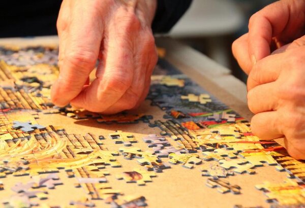
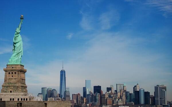
Now, let’s say we also have this feature.

Can you recognize what this object is?
Many Americans and people who have traveled to New York City would guess that this is the Statue of Liberty. And in fact, it is.
With just two features, you were able to identify this object. Computers follow a similar process when you run a feature detection algorithm to perform object recognition.
The Python computer vision library OpenCV has a number of algorithms to detect features in an image. We will explore these algorithms in this tutorial.
Installation and Setup
Before we get started, let’s make sure we have all the software packages installed. Check to see if you have OpenCV installed on your machine. If you are using Anaconda, you can type:
conda install -c conda-forge opencv
Alternatively, you can type:
pip install opencv-python
Install Numpy, the scientific computing library.
pip install numpy
Install Matplotlib, the plotting library.
pip install matplotlib
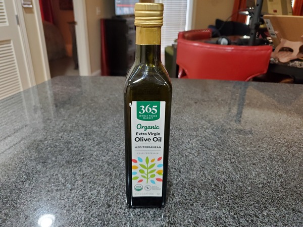
Find an Image File
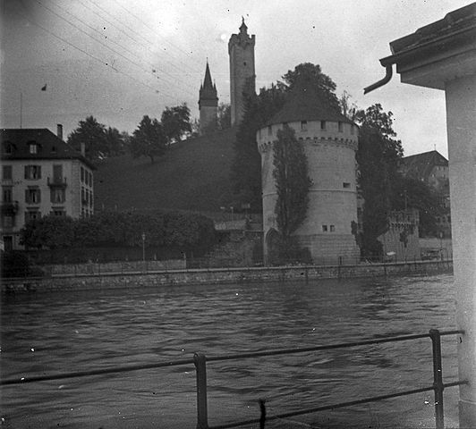
Find an image of any size. Here is mine:

Difference Between a Feature Detector and a Feature Descriptor
Before we get started developing our program, let’s take a look at some definitions.
The algorithms for features fall into two categories: feature detectors and feature descriptors.
A feature detector finds regions of interest in an image. The input into a feature detector is an image, and the output are pixel coordinates of the significant areas in the image.
A feature descriptor encodes that feature into a numerical “fingerprint”. Feature description makes a feature uniquely identifiable from other features in the image.
We can then use the numerical fingerprint to identify the feature even if the image undergoes some type of distortion.
Feature Detection Algorithms
Harris Corner Detection
A corner is an area of an image that has a large variation in pixel color intensity values in all directions. One popular algorithm for detecting corners in an image is called the Harris Corner Detector.
Here is some basic code for the Harris Corner Detector. I named my file harris_corner_detector.py.
# Code Source: https://opencv-python-tutroals.readthedocs.io/en/latest/py_tutorials/py_feature2d/py_features_harris/py_features_harris.html

import cv2
import numpy as np

filename = 'random-shapes-small.jpg'
img = cv2.imread(filename)
gray = cv2.cvtColor(img,cv2.COLOR_BGR2GRAY)

gray = np.float32(gray)
dst = cv2.cornerHarris(gray,2,3,0.04)

#result is dilated for marking the corners, not important
dst = cv2.dilate(dst,None)

# Threshold for an optimal value, it may vary depending on the image.
img[dst>0.01*dst.max()]=[0,0,255]

cv2.imshow('dst',img)
if cv2.waitKey(0) & 0xff == 27:
    cv2.destroyAllWindows()
Here is my image before:

Here is my image after:

For a more detailed example, check out my post “Detect the Corners of Objects Using Harris Corner Detector.”
Shi-Tomasi Corner Detector and Good Features to Track
Another corner detection algorithm is called Shi-Tomasi. Let’s run this algorithm on the same image and see what we get. Here is the code. I named the file shi_tomasi_corner_detect.py.
# Code Source: https://opencv-python-tutroals.readthedocs.io/en/latest/py_tutorials/py_feature2d/py_shi_tomasi/py_shi_tomasi.html

import numpy as np
import cv2
from matplotlib import pyplot as plt

img = cv2.imread('random-shapes-small.jpg')
gray = cv2.cvtColor(img,cv2.COLOR_BGR2GRAY)

# Find the top 20 corners
corners = cv2.goodFeaturesToTrack(gray,20,0.01,10)
corners = np.int0(corners)

for i in corners:
    x,y = i.ravel()
    cv2.circle(img,(x,y),3,255,-1)

cv2.imshow('Shi-Tomasi', img)
cv2.waitKey(0)
cv2.destroyAllWindows()
Here is the image after running the program:

Scale-Invariant Feature Transform (SIFT)
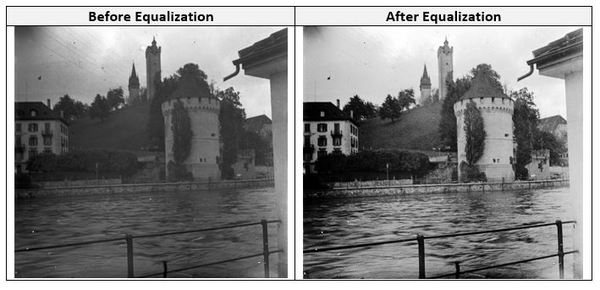
When we rotate an image or change its size, how can we make sure the features don’t change? The methods I’ve used above aren’t good at handling this scenario.
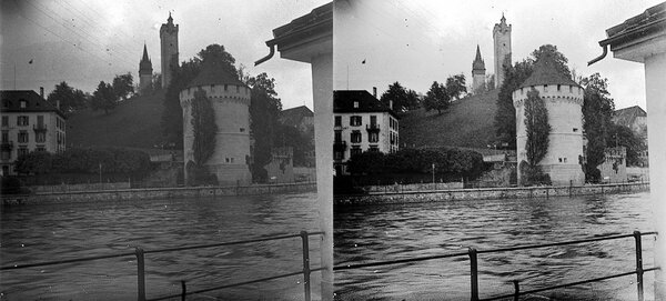
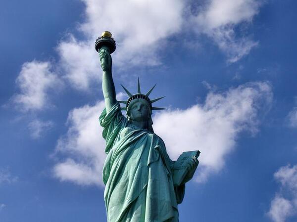
For example, consider these three images below of the Statue of Liberty in New York City. You know that this is the Statue of Liberty regardless of changes in the angle, color, or rotation of the statue in the photo. However, computers have a tough time with this task.


OpenCV has an algorithm called SIFT that is able to detect features in an image regardless of changes to its size or orientation. This property of SIFT gives it an advantage over other feature detection algorithms which fail when you make transformations to an image.
Here is an example of code that uses SIFT:
# Code source: https://docs.opencv.org/master/da/df5/tutorial_py_sift_intro.html
import numpy as np
import cv2 as cv
# Read the image
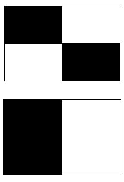
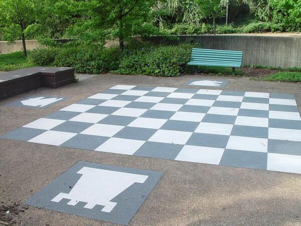
img = cv.imread('chessboard.jpg')
# Convert to grayscale
gray = cv.cvtColor(img,cv.COLOR_BGR2GRAY)
# Find the features (i.e. keypoints) and feature descriptors in the image
sift = cv.SIFT_create()
kp, des = sift.detectAndCompute(gray,None)
# Draw circles to indicate the location of features and the feature's orientation
img=cv.drawKeypoints(gray,kp,img,flags=cv.DRAW_MATCHES_FLAGS_DRAW_RICH_KEYPOINTS)
# Save the image
cv.imwrite('sift_with_features_chessboard.jpg',img)
Here is the before:
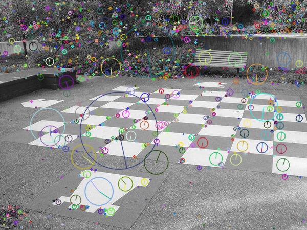
Here is the after. Each of those circles indicates the size of that feature. The line inside the circle indicates the orientation of the feature:
Speeded-up robust features (SURF)
SURF is a faster version of SIFT. It is another way to find features in an image.
Here is the code:
# Code Source: https://docs.opencv.org/master/df/dd2/tutorial_py_surf_intro.html

import numpy as np
import cv2 as cv

# Read the image
img = cv.imread('chessboard.jpg')

# Find the features (i.e. keypoints) and feature descriptors in the image
surf = cv.xfeatures2d.SURF_create(400)
kp, des = sift.detectAndCompute(img,None)

# Draw circles to indicate the location of features and the feature's orientation
img=cv.drawKeypoints(gray,kp,img,flags=cv.DRAW_MATCHES_FLAGS_DRAW_RICH_KEYPOINTS)

# Save the image
cv.imwrite('surf_with_features_chessboard.jpg',img)
Features from Accelerated Segment Test (FAST)
A lot of the feature detection algorithms we have looked at so far work well in different applications. However, they aren’t fast enough for some robotics use cases (e.g. SLAM).
The FAST algorithm, implemented here, is a really fast algorithm for detecting corners in an image.
Blob Detectors With LoG, DoG, and DoH
A blob is another type of feature in an image. A blob is a region in an image with similar pixel intensity values. Another definition you will hear is that a blob is a light on dark or a dark on light area of an image.
Three popular blob detection algorithms are Laplacian of Gaussian (LoG), Difference of Gaussian (DoG), and Determinant of Hessian (DoH).
Basic implementations of these blob detectors are at this page on the scikit-image website. Scikit-image is an image processing library for Python.
Feature Descriptor Algorithms
Histogram of Oriented Gradients
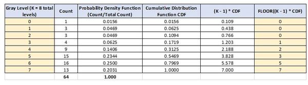
The HoG algorithm breaks an image down into small sections and calculates the gradient and orientation in each section. This information is then gathered into bins to compute histograms. These histograms give an image numerical “fingerprints” that make it uniquely identifiable.
A basic implementation of HoG is at this page.
Binary Robust Independent Elementary Features (BRIEF)
BRIEF is a fast, efficient alternative to SIFT. A sample implementation of BRIEF is here at the OpenCV website.
Oriented FAST and Rotated BRIEF (ORB)
SIFT was patented for many years, and SURF is still a patented algorithm. ORB was created in 2011 as a free alternative to these algorithms. It combines the FAST and BRIEF algorithms. You can find a basic example of ORB at the OpenCV website.
Feature Matching Example
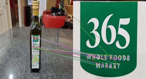
You can use ORB to locate features in an image and then match them with features in another image.
For example, consider this Whole Foods logo. This logo will be our training image.
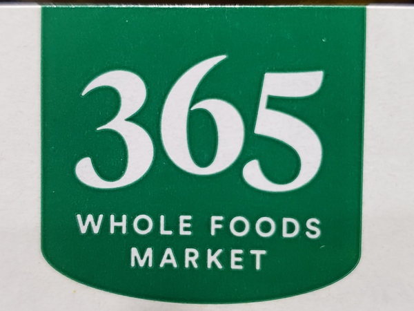
I want to locate this Whole Foods logo inside this image below. This image below is our query image.
Here is the code you need to run. My file is called feature_matching_orb.py.
import numpy as np
import cv2
from matplotlib import pyplot as plt

# Read the training and query images
query_img = cv2.imread('query_image.jpg')
train_img = cv2.imread('training_image.jpg')

# Convert the images to grayscale
query_img_gray = cv2.cvtColor(query_img,cv2.COLOR_BGR2GRAY)
train_img_gray = cv2.cvtColor(train_img, cv2.COLOR_BGR2GRAY)

# Initialize the ORB detector algorithm
orb = cv2.ORB_create()

# Detect keypoints (features) cand calculate the descriptors
query_keypoints, query_descriptors = orb.detectAndCompute(query_img_gray,None)
train_keypoints, train_descriptors = orb.detectAndCompute(train_img_gray,None)

# Match the keypoints
matcher = cv2.BFMatcher()
matches = matcher.match(query_descriptors,train_descriptors)

# Draw the keypoint matches on the output image
output_img = cv2.drawMatches(query_img, query_keypoints,
train_img, train_keypoints, matches[:20],None)

output_img = cv2.resize(output_img, (1200,650))

# Save the final image
cv2.imwrite("feature_matching_result.jpg", output_img)

# Close OpenCV upon keypress
cv2.waitKey(0)
cv2.destroyAllWindows()
Here is the result:
If you want to dive deeper into feature matching algorithms (Homography, RANSAC, Brute-Force Matcher, FLANN, etc.), check out the official tutorials on the OpenCV website. This page and this page have some basic examples.
That’s it. Keep building!