In this tutorial, we’ll learn the basics of how to interface ROS 2 Galactic with OpenCV, the popular computer vision library. These basics will provide you with the foundation to add vision to your robotics applications.
We’ll create an image publisher node to publish webcam data (i.e. video frames) to a topic, and we’ll create an image subscriber node that subscribes to that topic.
If you’re interested in integrating OpenCV with ROS 2 Foxy, check out this tutorial.
Prerequisites
- ROS 2 Galactic installed on Ubuntu Linux 20.04
- You have already created a ROS 2 workspace. The name of my workspace is dev_ws.
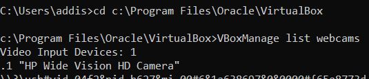
- You have a working webcam that is connected and tested on your Ubuntu installation.
- You are able to run the code on this tutorial on your Ubuntu machine without any problems.
You can find all the code for this project at this link on my Google Drive.
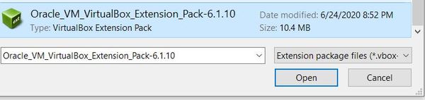
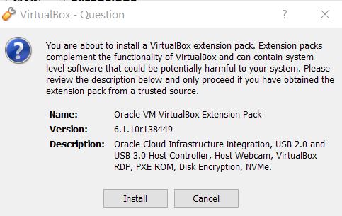
Connect Your Built-in Webcam to Ubuntu 20.04 on a VirtualBox and Test OpenCV
Follow this tutorial to connect your built-in webcam to Ubuntu 20.04 on a Virtual Box and to test OpenCV on your machine.
Create a Package
Open a new terminal window, and navigate to the src directory of your workspace:
cd ~/dev_ws/src
Now let’s create a package named opencv_tools (you can name the package anything you want).
Type this command (this is all a single command):
ros2 pkg create --build-type ament_python opencv_tools --dependencies rclpy image_transport cv_bridge sensor_msgs std_msgs opencv2
Modify Package.xml
Go to the dev_ws/src/cv_basics folder.
cd ~/dev_ws/src/cv_basics
Make sure you have a text editor installed. I like to use gedit.
sudo apt-get install gedit
Open the package.xml file.
gedit package.xml
Fill in the description of the cv_basics package, your email address and name on the maintainer line, and the license you desire (e.g. Apache License 2.0).
<description>Basic OpenCV-ROS2 nodes</description>
<maintainer email="automaticaddison@todo.todo">automaticaddison</maintainer>
<license>Apache License 2.0</license>
Save and close the file.
Build a Package
Return to the root of your workspace:
cd ~/dev_ws/
Build all packages in the workspace.
colcon build
Create the Image Publisher Node (Python)
Open a new terminal window, and type:
cd ~/dev_ws/src/opencv_tools/opencv_tools
Open a new Python file named basic_image_publisher.py.
gedit basic_image_publisher.py
Type the code below into it:
# Basic ROS 2 program to publish real-time streaming
# video from your built-in webcam
# Author:
# - Addison Sears-Collins
# - https://automaticaddison.com
# Import the necessary libraries
import rclpy # Python Client Library for ROS 2
from rclpy.node import Node # Handles the creation of nodes
from sensor_msgs.msg import Image # Image is the message type
from cv_bridge import CvBridge # Package to convert between ROS and OpenCV Images
import cv2 # OpenCV library
class ImagePublisher(Node):
"""
Create an ImagePublisher class, which is a subclass of the Node class.
"""
def __init__(self):
"""
Class constructor to set up the node
"""
# Initiate the Node class's constructor and give it a name
super().__init__('image_publisher')
# Create the publisher. This publisher will publish an Image
# to the video_frames topic. The queue size is 10 messages.
self.publisher_ = self.create_publisher(Image, 'video_frames', 10)
# We will publish a message every 0.1 seconds
timer_period = 0.1 # seconds
# Create the timer
self.timer = self.create_timer(timer_period, self.timer_callback)
# Create a VideoCapture object
# The argument '0' gets the default webcam.
self.cap = cv2.VideoCapture(0)
# Used to convert between ROS and OpenCV images
self.br = CvBridge()
def timer_callback(self):
"""
Callback function.
This function gets called every 0.1 seconds.
"""
# Capture frame-by-frame
# This method returns True/False as well
# as the video frame.
ret, frame = self.cap.read()
if ret == True:
# Publish the image.
# The 'cv2_to_imgmsg' method converts an OpenCV
# image to a ROS 2 image message
self.publisher_.publish(self.br.cv2_to_imgmsg(frame))
# Display the message on the console
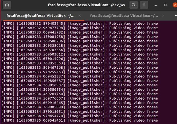
self.get_logger().info('Publishing video frame')
def main(args=None):
# Initialize the rclpy library
rclpy.init(args=args)
# Create the node
image_publisher = ImagePublisher()
# Spin the node so the callback function is called.
rclpy.spin(image_publisher)
# Destroy the node explicitly
# (optional - otherwise it will be done automatically
# when the garbage collector destroys the node object)
image_publisher.destroy_node()
# Shutdown the ROS client library for Python
rclpy.shutdown()
if __name__ == '__main__':
main()
Save and close the editor.
Modify Setup.py
Go to the following directory.
cd ~/dev_ws/src/opencv_tools/
Open setup.py.
gedit setup.py
Add the following line between the ‘console_scripts’: brackets:
'img_publisher = opencv_tools.basic_image_publisher:main',
The whole block should look like this:
entry_points={
    'console_scripts': [
      'img_publisher = opencv_tools.basic_image_publisher:main',
    ],
},
Save the file, and close it.
Create the Image Subscriber Node (Python)
Open a new terminal window, and type:
cd ~/dev_ws/src/opencv_tools/opencv_tools
Open a new Python file named basic_image_subscriber.py.
gedit basic_image_subscriber.py
Type the code below into it:
# Basic ROS 2 program to subscribe to real-time streaming
# video from your built-in webcam
# Author:
# - Addison Sears-Collins
# - https://automaticaddison.com
# Import the necessary libraries
import rclpy # Python library for ROS 2
from rclpy.node import Node # Handles the creation of nodes
from sensor_msgs.msg import Image # Image is the message type
from cv_bridge import CvBridge # Package to convert between ROS and OpenCV Images
import cv2 # OpenCV library
class ImageSubscriber(Node):
"""
Create an ImageSubscriber class, which is a subclass of the Node class.
"""
def __init__(self):
"""
Class constructor to set up the node
"""
# Initiate the Node class's constructor and give it a name
super().__init__('image_subscriber')
# Create the subscriber. This subscriber will receive an Image
# from the video_frames topic. The queue size is 10 messages.
self.subscription = self.create_subscription(
Image,
'video_frames',
self.listener_callback,
10)
self.subscription # prevent unused variable warning
# Used to convert between ROS and OpenCV images
self.br = CvBridge()
def listener_callback(self, data):
"""
Callback function.
"""
# Display the message on the console
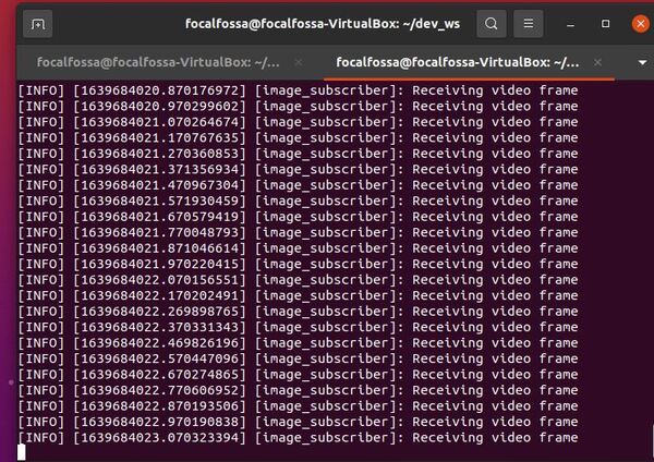
self.get_logger().info('Receiving video frame')
# Convert ROS Image message to OpenCV image
current_frame = self.br.imgmsg_to_cv2(data)
# Display image
cv2.imshow("camera", current_frame)
cv2.waitKey(1)
def main(args=None):
# Initialize the rclpy library
rclpy.init(args=args)
# Create the node
image_subscriber = ImageSubscriber()
# Spin the node so the callback function is called.
rclpy.spin(image_subscriber)
# Destroy the node explicitly
# (optional - otherwise it will be done automatically
# when the garbage collector destroys the node object)
image_subscriber.destroy_node()
# Shutdown the ROS client library for Python
rclpy.shutdown()
if __name__ == '__main__':
main()
Save and close the editor.
Modify Setup.py
Go to the following directory.
cd ~/dev_ws/src/opencv_tools/
Open setup.py.
gedit setup.py
Make sure the entry_points block looks like this:
entry_points={
    'console_scripts': [
      'img_publisher = opencv_tools.basic_image_publisher:main',
      'img_subscriber = opencv_tools.basic_image_subscriber:main',
    ],
},
Save the file, and close it.
Build the Package
Return to the root of your workspace:
cd ~/dev_ws/
We need to double check that all the dependencies needed are already installed.
rosdep install -i --from-path src --rosdistro galactic -y
If you get the following error:
ERROR: the following packages/stacks could not have their rosdep keys resolved to system dependencies: cv_basics: Cannot locate rosdep definition for [opencv2]
To resolve the error, open your package.xml file.
cd ~/dev_ws/src/opencv_tools/
gedit package.xml
Change “opencv2” in your package.xml to “opencv-python” so that rosdep can find it.
Save the file, and close it.
Build the package:
cd ~/dev_ws/
colcon build
Run the Nodes
To run the nodes, open a new terminal window.
Make sure you are in the root of your workspace:
cd ~/dev_ws/
Run the publisher node. If you recall, its name is img_publisher.
ros2 run opencv_tools img_publisher
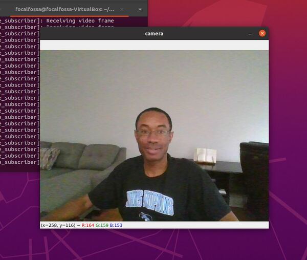
Open a new terminal, and run the subscriber node.
ros2 run opencv_tools img_subscriber
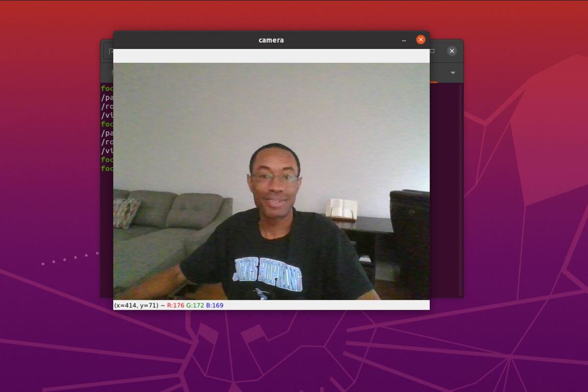
A window will pop up with the streaming video.
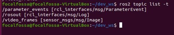
Check out the active topics.
ros2 topic list -t
See the relationship between the active nodes.
rqt_graph
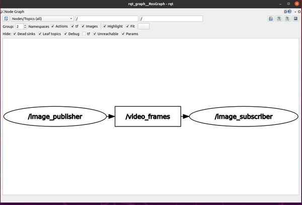
Click the refresh button. The refresh button is that circular arrow at the top of the screen.

Press CTRL+C in all terminal windows when you’re ready to shut everything down.
That’s it! Keep building!