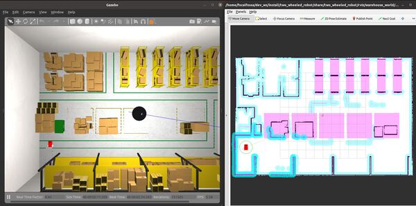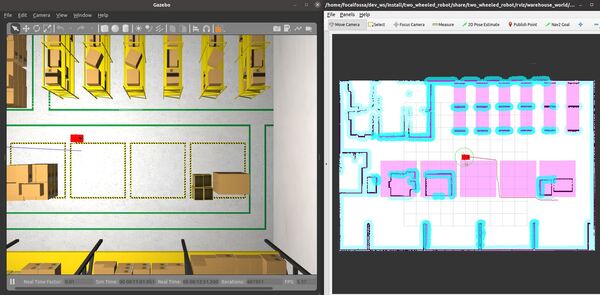
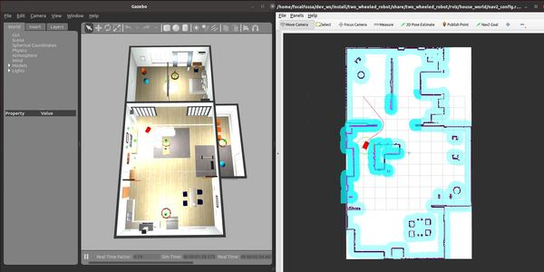
In this tutorial, I will show you how to command a simulated autonomous mobile robot to carry out an inspection task using the ROS 2 Navigation Stack (also known as Nav2). Here is the final output you will be able to achieve after going through this tutorial:
Real-World Applications
The application that we will develop in this tutorial can be used in a number of real-world robotic applications:
- Hospitals and Medical Centers
- Hotels (e.g. Room Service)
- House
- Offices
- Restaurants
- Warehouses
- And more…
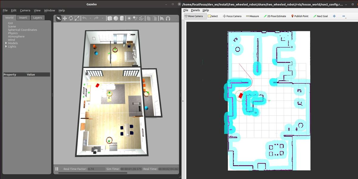
We will focus on creating an application that will enable a robot to perform an inspection inside a house.
Prerequisites
- ROS 2 Foxy Fitzroy installed on Ubuntu Linux 20.04 or newer. I am using ROS 2 Galactic, which is the latest version of ROS 2 as of the date of this post.
- You have already created a ROS 2 workspace. The name of our workspace is “dev_ws”, which stands for “development workspace.”
- You have Python 3.7 or higher.
- (Optional) You have completed my Ultimate Guide to the ROS 2 Navigation Stack.
- (Optional) You have a package named two_wheeled_robot inside your ~/dev_ws/src folder, which I set up in this post. If you have another package, that is fine.
- (Optional) You know how to load a world file into Gazebo using ROS 2.
You can find the files for this post here on my Google Drive. Credit to this GitHub repository for the code.
Create a World
Open a terminal window, and move to your package.
cd ~/dev_ws/src/two_wheeled_robot/worlds
Make sure this world is inside this folder. The name of the file is house.world.
Create a Map
Open a terminal window, and move to your package.
cd ~/dev_ws/src/two_wheeled_robot/maps/house_world
Make sure the pgm and yaml map files are inside this folder.
My world map is made up of two files:
- house_world.pgm
- house_world.yaml
Create the Parameters File
Let’s create the parameters file.
Open a terminal window, and move to your package.
cd ~/dev_ws/src/two_wheeled_robot/params/house_world
Add this file. The name of the file is nav2_params.yaml.
Create the RViz Configuration File
Let’s create the RViz configuration file.
Open a terminal window, and move to your package.
cd ~/dev_ws/src/two_wheeled_robot/rviz/house_world
Add this file. The name of the file is nav2_config.rviz.
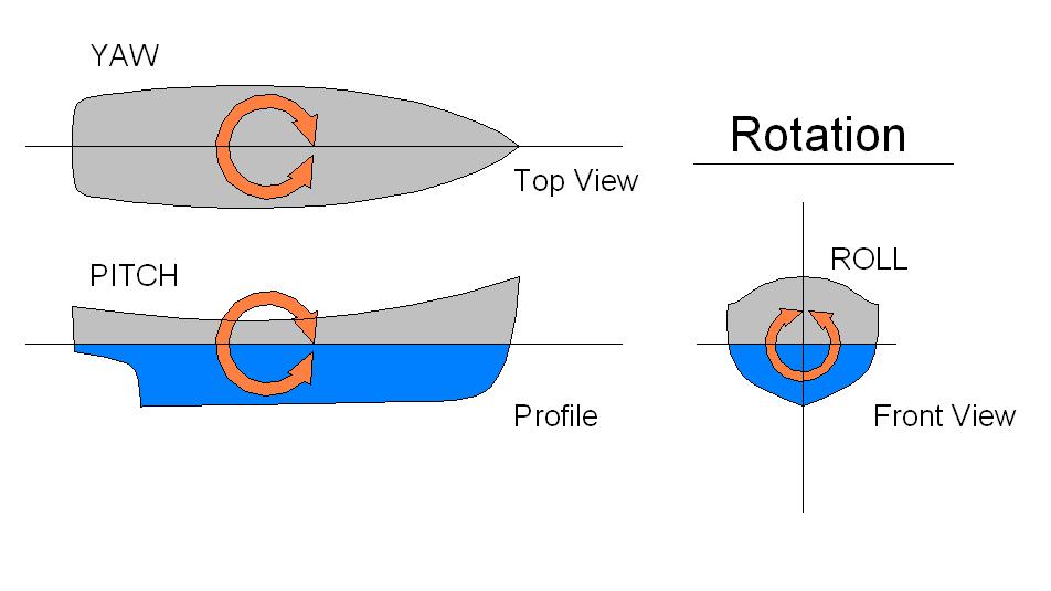
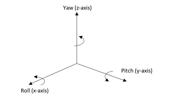
Create a Python Script to Convert Euler Angles to Quaternions
Let’s create a Python script to convert Euler angles to quaternions. We will need to use this script later.
Open a terminal window, and move to your package.
cd ~/dev_ws/src/two_wheeled_robot/two_wheeled_robot
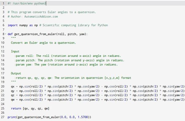
Open a new Python program called euler_to_quaternion.py.
gedit euler_to_quaternion.py
Add this code.
Save the code, and close the file.
Change the access permissions on the file.
chmod +x euler_to_quaternion.py
Since our script depends on NumPy, the scientific computing library for Python, we need to add it as a dependency to the package.xml file.
cd ~/dev_ws/src/two_wheeled_robot/
gedit package.xml
<exec_depend>python3-numpy</exec_depend>Here is the package.xml file. Add that code, and save the file.
To make sure you have NumPy, return to the terminal window, and install it.
sudo apt-get update
sudo apt-get upgrade
sudo apt install python3-numpy
Add the Python Script
Open a terminal window, and move to your package.
cd ~/dev_ws/src/two_wheeled_robot/scripts
Open a new Python program called run_inspection.py.
gedit run_inspection.py
Add this code.
Save the code, and close the file.
Change the access permissions on the file.
chmod +x run_inspection.py
Open a new Python program called robot_navigator.py.
gedit robot_navigator.py
Add this code.
Save the code and close the file.
Change the access permissions on the file.
chmod +x robot_navigator.py
Open CMakeLists.txt.
cd ~/dev_ws/src/two_wheeled_robot
gedit CMakeLists.txt
Add the Python executables.
scripts/run_inspection.py
scripts/robot_navigator.py
Create a Launch File
cd ~/dev_ws/src/two_wheeled_robot/launch/house_world
gedit house_world_inspection.launch.py
Save and close.
Build the Package
Now we build the package.
cd ~/dev_ws/
colcon build
Open a new terminal and launch the robot.
ros2 launch two_wheeled_robot house_world_inspection.launch.py
Now command the robot to perform the house inspection by opening a new terminal window, and typing:
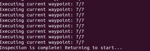
ros2 run two_wheeled_robot run_inspection.py
The robot will perform the inspection.
To modify the coordinates of the waypoints located in the run_inspection.py file, you can use the Publish Point button in RViz and look at the output in the terminal window by observing the clicked_point topic.
ros2 topic echo /clicked_point
Each time you click on an area, the coordinate will publish to the terminal window.
Also, if you want to run a node that runs in a loop (e.g. a security patrol demo), you can use this code.
To run that node, you would type:
ros2 run two_wheeled_robot security_demo.py
That’s it! Keep building!