In this project, I will show you how to display an image using OpenCV.
You Will Need
Python 3.7+
Directions
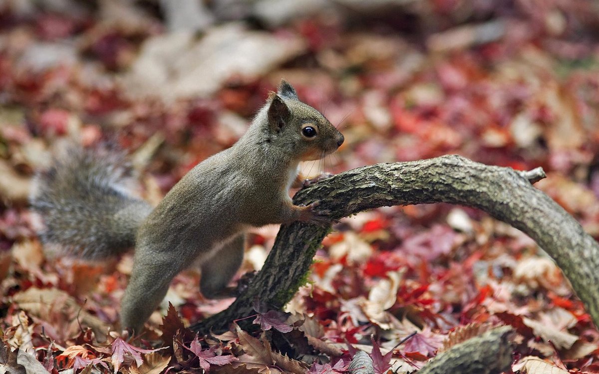
Let’s say you have an image like the one below. The file name is 1.jpg.
To display it using OpenCV, go to your favorite IDE or text editor and create the following Python program:
# Display a color image using OpenCV
import numpy as np
import cv2

# Load an color image in grayscale
img = cv2.imread('1.jpg',1)

cv2.imshow('image',img)
cv2.waitKey(0)
cv2.destroyAllWindows()
Save the program into the same directory as 1.jpg.
Run the file.
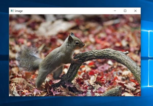
Watch the image display to your computer. That’s it!
In this post, I will show you how to install TensorFlow 2 on Windows 10. TensorFlow2 is a free software library used for machine learning applications. It comes integrated with Keras, a neural-network library written in Python. If you want to work with neural networks and deep learning, TensorFlow 2 should be your software of choice because of its popularity both in academia and in industry. Let’s get started!
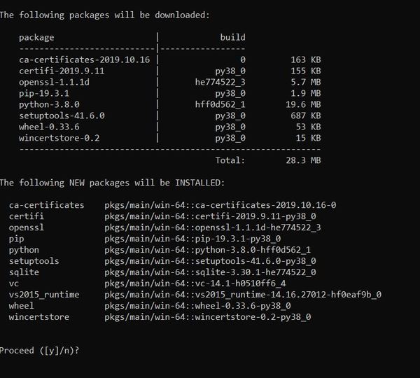
Type the command below to create a virtual environment named tf_2 with the latest version of Python installed. A virtual environment is like an independent Python workspace which has its own set of libraries and Python version installed. For example, you might have a project that needs to run using an older version of Python, like Python 2.7. You might have another project that requires Python 3.7. You can create separate virtual environments for these projects.
conda create -n tf_2 python
Press y and then ENTER.
Wait for the software to download.
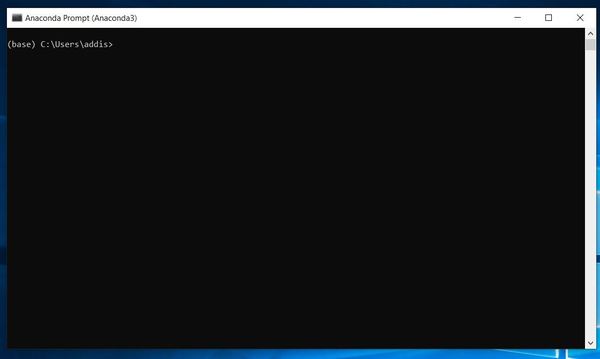
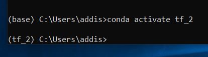
Once the download is finished, activate the virtual environment using this command:
conda activate tf_2
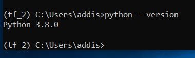
Check which version of Python you have installed on your system. I have Python 3.8.0.
python --version
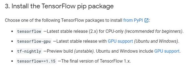
Choose a TensorFlow package. I’ll install TensorFlow CPU. Let’s type the following command:
pip install --upgrade tensorflow
You might see this error:
ERROR: Could not find a version that satisfies the requirement tensorflow (from versions: none)
ERROR: No matching distribution found for tensorflow
If you do, you need to downgrade your version of Python. TensorFlow is not yet compatible with your newest version of Python.
conda install python=3.6
Press y and then ENTER.
Check which version of Python you have installed on your system. I have Python 3.6.9 now.
python --version
Now install TensorFlow 2.
pip install --upgrade tensorflow
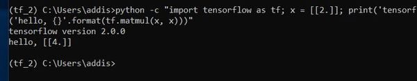
Wait for Tensorflow CPU to finish installing. Once it is finished installing, verify the installation by typing:
python -c "import tensorflow as tf; x = [[2.]]; print('tensorflow version', tf.__version__); print('hello, {}'.format(tf.matmul(x, x)))"
Here is the output:
You should see your TensorFlow version in the output.
You might see this message:
“I tensorflow/core/platform/cpu_feature_guard.cc:142] Your CPU supports instructions that this TensorFlow binary was not compiled to use: AVX2”
Don’t worry, TensorFlow is working just fine. To get rid of that message, you can set the environment variables inside the virtual environment. Type the following command:
set TF_CPP_MIN_LOG_LEVEL=2
Now run this command:
python -c "import tensorflow as tf; x = [[2.]]; print('tensorflow version', tf.__version__); print('hello, {}'.format(tf.matmul(x, x)))"
I’m now going to open up a text editor and type a Python program. I will save it to my D drive as fashion_mnist.py. Here is the code:
from __future__ import absolute_import, division, print_function, unicode_literals

# Import the key libraries
import matplotlib.pyplot as plt
import tensorflow as tf
import numpy as np

# Rename tf.keras.layers
layers = tf.keras.layers

# Print the TensorFlow version
print(tf.__version__)

# Load and prepare the MNIST dataset.
# Convert the samples from integers to floating-point numbers:
mnist = tf.keras.datasets.fashion_mnist
(x_train, y_train), (x_test, y_test) = mnist.load_data()
x_train, x_test = x_train / 255.0, x_test / 255.0

# Let's plot the data so we can see it
class_names = ['T-shirt/top', 'Trouser', 'Pullover', 'Dress', 'Coat', 'Sandal',
 'Shirt', 'Sneaker', 'Bag', 'Ankle boot']
plt.figure(figsize=(10,10))

for i in range(25):
 plt.subplot(5,5,i+1)
 plt.xticks([])
 plt.yticks([])
 plt.grid(False)
 plt.imshow(x_train[i], cmap=plt.cm.binary)
 plt.xlabel(class_names[y_train[i]])
plt.show()
Within your virtual environment in the Anaconda terminal, navigate to where you saved your code. I will type.
D:
Then:
cd D:\<YOUR_PATH>\install_tensorflow2
Type dir to see if the Python (.py) file is in that directory.
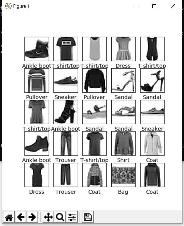
Now run the code:
python fashion_mnist.py
You should see this graphic pop up.
In the terminal window, press CTRL+C on your keyboard to stop the code from running.
Let’s add to our code. Open up the Python file again in the text editor and type the following code. If you are new to neural networks, don’t worry what everything means at this stage.
from __future__ import absolute_import, division, print_function, unicode_literals

# Import the key libraries
import matplotlib.pyplot as plt
import tensorflow as tf
import numpy as np

# Rename tf.keras.layers
layers = tf.keras.layers

# Print the TensorFlow version
print(tf.__version__)

# Load and prepare the MNIST dataset.
# Convert the samples from integers to floating-point numbers:
mnist = tf.keras.datasets.fashion_mnist
(x_train, y_train), (x_test, y_test) = mnist.load_data()
x_train, x_test = x_train / 255.0, x_test / 255.0

# Let's plot the data so we can see it
class_names = ['T-shirt/top', 'Trouser', 'Pullover', 'Dress', 'Coat', 'Sandal',
 'Shirt', 'Sneaker', 'Bag', 'Ankle boot']
plt.figure(figsize=(10,10))

for i in range(25):
 plt.subplot(5,5,i+1)
 plt.xticks([])
 plt.yticks([])
 plt.grid(False)
 plt.imshow(x_train[i], cmap=plt.cm.binary)
 plt.xlabel(class_names[y_train[i]])
plt.show()

# Build the neural network layer-by-layer
model = tf.keras.Sequential()
model.add(layers.Flatten()) # Make the input layer one-dimensional
model.add(layers.Dense(64, activation='relu')) # Layer has 64 nodes; Uses ReLU
model.add(layers.Dense(64, activation='relu')) # Layer has 64 nodes; Uses ReLU
model.add(layers.Dense(10, activation='softmax')) # Layer has 64 nodes; Uses Softmax

# Choose an optimizer and loss function for training:
model.compile(optimizer='adam',
 loss='sparse_categorical_crossentropy',
 metrics=['accuracy'])

# Train and evaluate the model's accuracy
model.fit(x_train, y_train, epochs=5)
model.evaluate(x_test,  y_test, verbose=2)
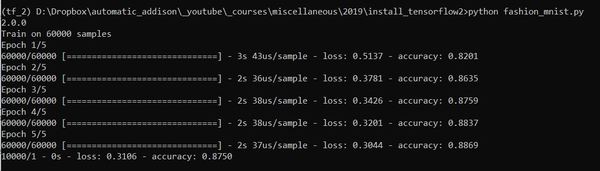
Run the code:
python fashion_mnist.py
When you see the plot of the clothes appear, just close that window so that the neural network build and run.
Here is the output.
The accuracy of classifying the clothing items was 87.5%. Pretty cool huh! Congratulations! You’ve built and run your first neural network on TensorFlow 2.
To deactivate the virtual environment, type:
conda deactivate
Then to exit the terminal, type:
exit
At this stage, I encourage you to go through the TensorFlow tutorials to get more practice using this really powerful tool.
First, before we get into the pros and cons of Gaussian smoothing, let us take a quick look at what Gaussian smoothing is and why we use it.
What is Gaussian Smoothing?
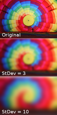
Have you ever had a photo or portrait of either yourself or someone else and wanted to smooth out the facial imperfections, pimples, pores, or wrinkles? Gaussian smoothing (also known as Gaussian blur) is one way to do this. Gaussian smoothing uses a mathematical equation called the Gaussian function to blur an image, reducing image detail and noise.
Below is an example of an image with a small and large Gaussian blur.
Noise reduction is one of the main use cases of Gaussian smoothing.
Easy to implement
No complicated algorithms with multiple nested for loops needed. As you can see in this MATLAB implementation, Gaussian smoothing can be done with just a single line of code.
Automatic censoring
Some use cases might require you to conceal the identity of someone or to censor images that might contain material that might be inappropriate to certain audiences. Gaussian smoothing works well in these cases.
Symmetric
Gaussian smoothing produces an image that is rotationally symmetric. It is applied the same no matter what direction you go in.
Cons of Gaussian Smoothing
Lose fine image detail and contrast
If you have a use case that requires you to examine fine detail, Gaussian smoothing might make that a lot harder. An example where you might want to examine fine detail would be in a medical image or a robot trying to grasp a specific point on an object.
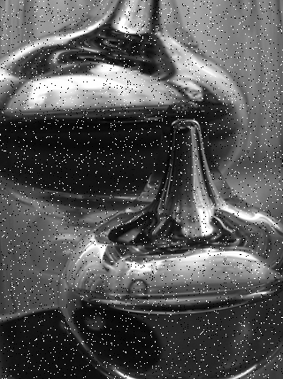
Does not handle “salt and pepper noise” well
Sometimes an image might have what is known as “salt-and-pepper noise.” Salt-and-pepper noise is defined as sparsely occurring white and black pixels. Below is an image showing salt-and-pepper noise.


