In this tutorial, we’ll learn the basics of how to interface ROS with OpenCV, the popular real-time computer vision library. These basics will provide you with the foundation to add vision to your robotics applications.
We’ll create an image publisher node to publish webcam data to a topic, and we’ll create an image subscriber node that subscribes to that topic.
The official tutorial is here at the ROS website, but we’ll run through the steps of a basic example below.
Connect Your Built-in Webcam to Ubuntu 20.04 on a VirtualBox
The first thing you need to do is make sure a camera is connected to your Ubuntu installation, and make sure the camera is turned on in Ubuntu. If you are using Ubuntu in a VirtualBox on a Windows machine, you can follow these steps.
Create a New ROS Package
Let’s create a new package named cv_basics.
Open up a terminal window, and type these two commands, one right after the other:
cd ~/catkin_ws/src
catkin_create_pkg cv_basics image_transport cv_bridge sensor_msgs rospy roscpp std_msgs
Create the Image Publisher Node (Python)
Change to the cv_basics package
roscd cv_basics
Create a directory for Python scripts.
mkdir scripts
Go into the scripts folder.
cd scripts
Open a new Python file named webcam_pub.py.
gedit webcam_pub.py
Type the code below into it:
#!/usr/bin/env python3
# Basics ROS program to publish real-time streaming
# video from your built-in webcam
# Author:
# - Addison Sears-Collins
# - https://automaticaddison.com

# Import the necessary libraries
import rospy # Python library for ROS
from sensor_msgs.msg import Image # Image is the message type
from cv_bridge import CvBridge # Package to convert between ROS and OpenCV Images
import cv2 # OpenCV library

def publish_message():

  # Node is publishing to the video_frames topic using
  # the message type Image
  pub = rospy.Publisher('video_frames', Image, queue_size=10)

  # Tells rospy the name of the node.
  # Anonymous = True makes sure the node has a unique name. Random
  # numbers are added to the end of the name.
  rospy.init_node('video_pub_py', anonymous=True)

  # Go through the loop 10 times per second
  rate = rospy.Rate(10) # 10hz

  # Create a VideoCapture object
  # The argument '0' gets the default webcam.
  cap = cv2.VideoCapture(0)

  # Used to convert between ROS and OpenCV images
  br = CvBridge()

  # While ROS is still running.
  while not rospy.is_shutdown():

      # Capture frame-by-frame
      # This method returns True/False as well
      # as the video frame.
      ret, frame = cap.read()

      if ret == True:
        # Print debugging information to the terminal
        rospy.loginfo('publishing video frame')

        # Publish the image.
        # The 'cv2_to_imgmsg' method converts an OpenCV
        # image to a ROS image message
        pub.publish(br.cv2_to_imgmsg(frame))

      # Sleep just enough to maintain the desired rate
      rate.sleep()

if __name__ == '__main__':
  try:
    publish_message()
  except rospy.ROSInterruptException:
    pass
Save and close the editor.
Make the file an executable.
chmod +x webcam_pub.py
Create the Image Subscriber Node (Python)
Now, let’s create the subscriber node. We’ll name it webcam_sub.py.
gedit webcam_sub.py
Type the code below into it:
#!/usr/bin/env python3
# Description:
# - Subscribes to real-time streaming video from your built-in webcam.
#
# Author:
# - Addison Sears-Collins
# - https://automaticaddison.com

# Import the necessary libraries
import rospy # Python library for ROS
from sensor_msgs.msg import Image # Image is the message type
from cv_bridge import CvBridge # Package to convert between ROS and OpenCV Images
import cv2 # OpenCV library

def callback(data):

  # Used to convert between ROS and OpenCV images
  br = CvBridge()

  # Output debugging information to the terminal
  rospy.loginfo("receiving video frame")

  # Convert ROS Image message to OpenCV image
  current_frame = br.imgmsg_to_cv2(data)

  # Display image
  cv2.imshow("camera", current_frame)

  cv2.waitKey(1)

def receive_message():

  # Tells rospy the name of the node.
  # Anonymous = True makes sure the node has a unique name. Random
  # numbers are added to the end of the name.
  rospy.init_node('video_sub_py', anonymous=True)

  # Node is subscribing to the video_frames topic
  rospy.Subscriber('video_frames', Image, callback)

  # spin() simply keeps python from exiting until this node is stopped
  rospy.spin()

  # Close down the video stream when done
  cv2.destroyAllWindows()

if __name__ == '__main__':
  receive_message()
Save and close the editor.
Make the file an executable.
chmod +x webcam_sub.py
Build Both Nodes (Python)
Open a new terminal window, and type the following commands to build all the nodes in the package:
cd ~/catkin_ws
catkin_make
Launch Both Nodes (Python)
Now, let’s create a launch file that launches both the publisher and subscriber nodes.
Open a new terminal window, and go to your package.
roscd cv_basics
Create a new folder named launch.
mkdir launch
Move into the launch directory.
cd launch
Open a new file named cv_basics_py.launch.
gedit cv_basics_py.launch
Type the following code.
<launch>
  <node
    pkg="cv_basics"
    type="webcam_pub.py"
    name="webcam_pub"
    output="screen"
  />
  <node
    pkg="cv_basics"
    type="webcam_sub.py"
    name="webcam_sub"
    output="screen"
  />
</launch>
Save and close the editor.
Open a new terminal window, and launch the programs.
roslaunch cv_basics cv_basics_py.launch
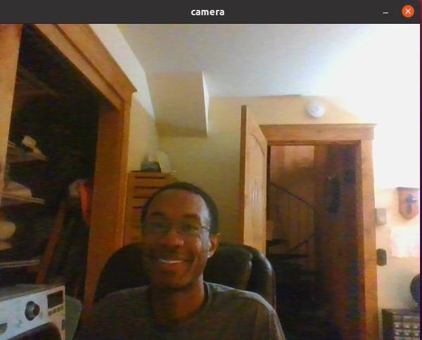
Here is the camera output you should see:
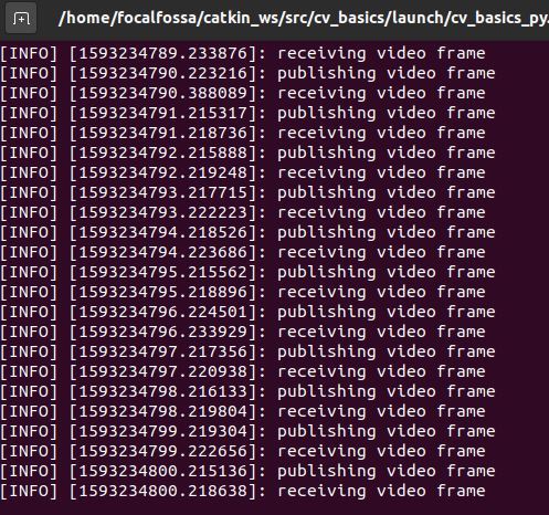
Here is the output to the terminal window.
Press CTRL+C when you’re ready to move on.
Create and Build the Image Publisher Node (C++)
C++ is really the recommended language for publishing and subscribing to images in ROS. The proper way to publish and subscribe to images in ROS is to use image_transport, a tool that provides support for transporting images in compressed formats that use less memory.
image_transport currently only works for C++. There is no support for Python yet.
Let’s build a publisher node that publishes real-time video to a ROS topic.
Go to your src folder of your package.
roscd cv_basics/src
Open a new C++ file named webcam_pub_cpp.cpp.
gedit webcam_pub_cpp.cpp
Type the code below.
#include <cv_bridge/cv_bridge.h>
#include <image_transport/image_transport.h>
#include <opencv2/highgui/highgui.hpp>
#include <ros/ros.h>
#include <sensor_msgs/image_encodings.h>

// Author: Addison Sears-Collins
// Website: https://automaticaddison.com
// Description: A basic image publisher for ROS in C++
// Date: June 27, 2020

int main(int argc, char** argv)
{
    ros::init(argc, argv, "video_pub_cpp");
    ros::NodeHandle nh;  // Default handler for nodes in ROS

    // 0 reads from your default camera
    const int CAMERA_INDEX = 0;
    cv::VideoCapture capture(CAMERA_INDEX);
    if (!capture.isOpened()) {
      ROS_ERROR_STREAM("Failed to open camera with index " << CAMERA_INDEX << "!");
      ros::shutdown();
    }

    // Image_transport is responsible for publishing and subscribing to Images
    image_transport::ImageTransport it(nh);

    // Publish to the /camera topic
    image_transport::Publisher pub_frame = it.advertise("camera", 1);

    cv::Mat frame;//Mat is the image class defined in OpenCV
    sensor_msgs::ImagePtr msg;

    ros::Rate loop_rate(10);

    while (nh.ok()) {

      // Load image
      capture >> frame;

      // Check if grabbed frame has content
      if (frame.empty()) {
        ROS_ERROR_STREAM("Failed to capture image!");
        ros::shutdown();
      }

      // Convert image from cv::Mat (OpenCV) type to sensor_msgs/Image (ROS) type and publish
      msg = cv_bridge::CvImage(std_msgs::Header(), "bgr8", frame).toImageMsg();
      pub_frame.publish(msg);
      /*
      Cv_bridge can selectively convert color and depth information. In order to use the specified
      feature encoding, there is a centralized coding form:
        Mono8: CV_8UC1, grayscale image
        Mono16: CV_16UC1, 16-bit grayscale image
        Bgr8: CV_8UC3 with color information and the order of colors is BGR order
        Rgb8: CV_8UC3 with color information and the order of colors is RGB order
        Bgra8: CV_8UC4, BGR color image with alpha channel
        Rgba8: CV_8UC4, CV, RGB color image with alpha channel
      */
      //cv::imshow("camera", image);
      cv::waitKey(1); // Display image for 1 millisecond

      ros::spinOnce();
      loop_rate.sleep();
    }

    // Shutdown the camera
    capture.release();
}
Save and close the editor.
Go to your CMakeLists.txt file inside your package.
roscd cv_basics
gedit CMakeLists.txt
This code goes under the find_package(catkin …) block.
find_package(OpenCV)
This code goes under the include_directories() block.
include_directories(${OpenCV_INCLUDE_DIRS})
This code goes at the bottom of the CMakeLists.txt file.
add_executable(webcam_pub_cpp src/webcam_pub_cpp.cpp)
target_link_libraries(webcam_pub_cpp ${catkin_LIBRARIES} ${OpenCV_LIBRARIES})
Save the file, and close it.
Open a new terminal window, and type the following commands to build all the nodes in the package:
cd ~/catkin_ws
catkin_make
Run the Image Publisher Node (C++)
Open a new terminal window, and launch the publisher node.
roscore
In another terminal tab, type:
rosrun cv_basics webcam_pub_cpp
You shouldn’t see anything printed to your terminal window.
To see the video frames that are getting published, type this command in yet another terminal tab. We can’t use the rostopic echo /camera command since it would spit out data that is not readable by humans.
You need to use a special node called the image_view node that displays images that are published to a specific topic (the /camera topic in our case).
rosrun image_view image_view image:=/camera
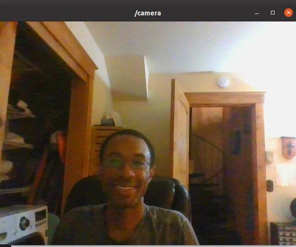
Here is what you should see:
Press CTRL+C to stop all the processes.
Create and Build the Image Subscriber Node (C++)
Go to your src folder of your package.
roscd cv_basics/src
Open a new C++ file named webcam_sub_cpp.cpp.
gedit webcam_sub_cpp.cpp
Type the code below.
#include <ros/ros.h>
#include <image_transport/image_transport.h>
#include <opencv2/highgui/highgui.hpp>
#include <cv_bridge/cv_bridge.h>

// Author: Addison Sears-Collins
// Website: https://automaticaddison.com
// Description: A basic image subscriber for ROS in C++
// Date: June 27, 2020

void imageCallback(const sensor_msgs::ImageConstPtr& msg)
{

  // Pointer used for the conversion from a ROS message to
  // an OpenCV-compatible image
  cv_bridge::CvImagePtr cv_ptr;

  try
  {

    // Convert the ROS message
    cv_ptr = cv_bridge::toCvCopy(msg, "bgr8");

    // Store the values of the OpenCV-compatible image
    // into the current_frame variable
    cv::Mat current_frame = cv_ptr->image;

    // Display the current frame
    cv::imshow("view", current_frame);

    // Display frame for 30 milliseconds
    cv::waitKey(30);
  }
  catch (cv_bridge::Exception& e)
  {
    ROS_ERROR("Could not convert from '%s' to 'bgr8'.", msg->encoding.c_str());
  }
}

int main(int argc, char **argv)
{
  // The name of the node
  ros::init(argc, argv, "frame_listener");

  // Default handler for nodes in ROS
  ros::NodeHandle nh;

  // Used to publish and subscribe to images
  image_transport::ImageTransport it(nh);

  // Subscribe to the /camera topic
  image_transport::Subscriber sub = it.subscribe("camera", 1, imageCallback);

  // Make sure we keep reading new video frames by calling the imageCallback function
  ros::spin();

  // Close down OpenCV
  cv::destroyWindow("view");
}
Save and close the editor.
Go to your CMakeLists.txt file inside your package.
roscd cv_basics
gedit CMakeLists.txt
Add this code to the bottom of the file.
add_executable(webcam_sub_cpp src/webcam_sub_cpp.cpp)
target_link_libraries(webcam_sub_cpp ${catkin_LIBRARIES} ${OpenCV_LIBRARIES})
Save the file, and close it.
Open a new terminal window, and type the following commands to build all the nodes in the package:
cd ~/catkin_ws
catkin_make
Launch Both Nodes (C++)
Go to your launch folder.
roscd cv_basics/launch
Open a new launch file.
gedit cv_basics_cpp.launch
Type the following code.
<launch>
  <node
    pkg="cv_basics"
    type="webcam_pub_cpp"
    name="webcam_pub_cpp"
    output="screen"
  />
  <node
    pkg="cv_basics"
    type="webcam_sub_cpp"
    name="webcam_sub_cpp"
    output="screen"
  />
</launch>
Save and close the editor.
Open a new terminal window, and launch the nodes.
roslaunch cv_basics cv_basics_cpp.launch
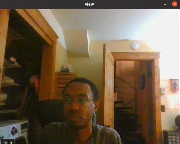
You should see output from the camera:
Press CTRL+C to stop all the processes.
That’s it. Keep building!