In this tutorial, I will show you everything you need to know to get started with the NVIDIA Jetson Nano. The official tutorial is here, but I will run through all the steps below. I recommend you go through these steps slowly. It took me a full day to set up the Jetson Nano, so be patient and enjoy the journey.
You Will Need
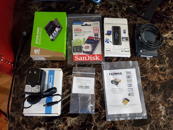
This section is the complete list of components you will need for this project (#ad).
Disclosure (#ad): As an Amazon Associate I earn from qualifying purchases.
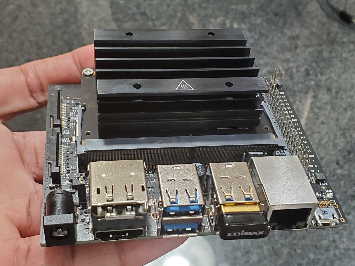
- NVIDIA Jetson Nano Developer Kit (4GB – B01)
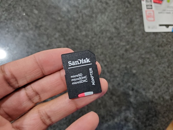
- 128GB MicroSD Card with Adapter
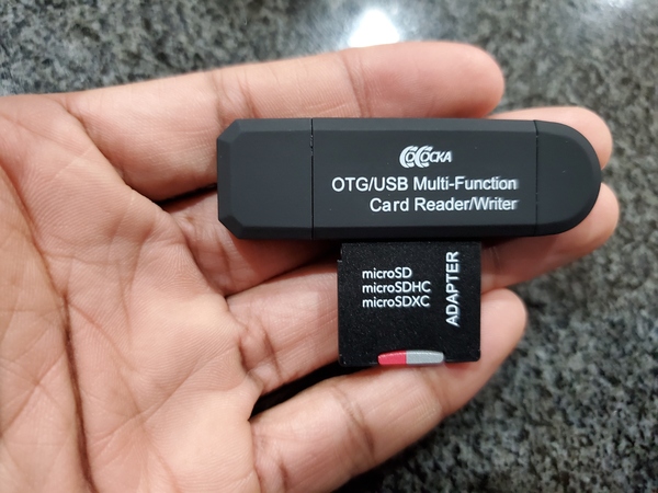
- SD/Micro SD Card Reader with Standard USB Connector
- USB to Micro-USB cable
- Power Supply Applicable for Jetson Nano 5V/4A OD 5.5mm ID 2.1mm
- 2.54mm Standard Computer Jumper Caps
- USB WiFi Adapter
- NVIDIA Jetson Cooling Fan and Case (Optional)
- USB keyboard
- USB mouse
- Computer monitor with an HDMI connection
Write the Operating System Image to the microSD Card
The first thing we need to do is to prepare the operating system. The Jetson Nano uses a microSD card for storing the operating system.
Grab your SD/Micro SD Card Reader with Standard USB Connector.
Grab your tiny 128GB MicroSD Card, and slide it into the adapter.
Put the adapter into the SD card reader.
Plug the SD card reader into your PC.
Check to see if the SD card reader appears in your lists of disks. Make a note of where this is on your PC. My SD card reader shows up as my F drive.
Download the Jetson Nano Developer Kit SD card image file (often called “JetPack”) to your PC. Mine will save to my Desktop. It is a large file and will take a long time to download. Just go get something to eat and come back when it is finished.
Now, we need to write the image to our microSD card. The instructions will vary depending if you have Windows, Mac OS, or Linux. I have a Windows PC, so here is what I will do next.
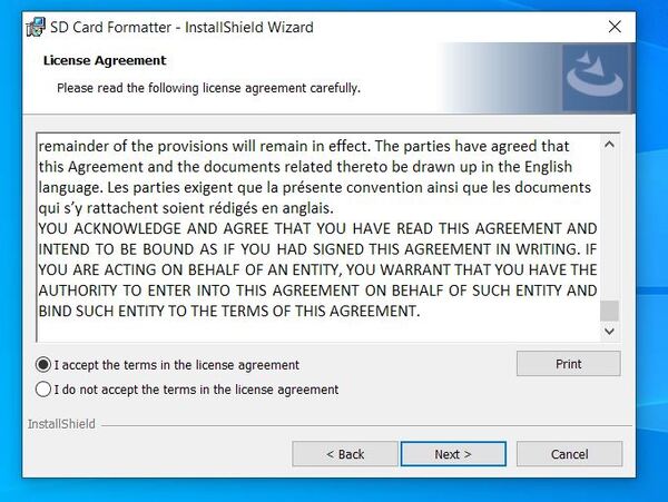
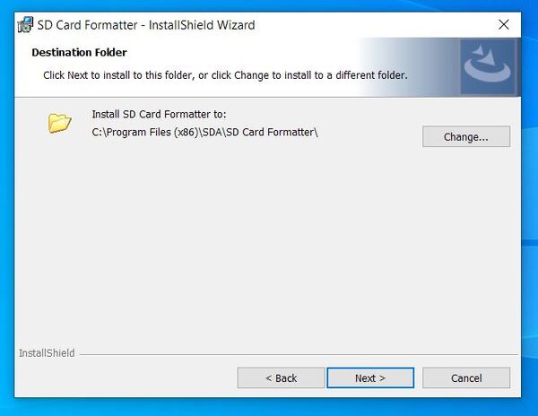
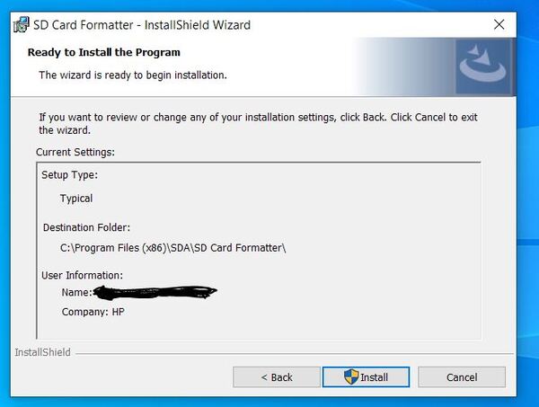
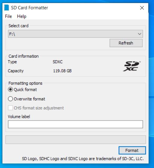
Download, install, and launch the SD Memory Card Formatter for Windows.
- Select the drive where your SD card reader is.
- Select “Quick format”.
- Leave “Volume label” blank.
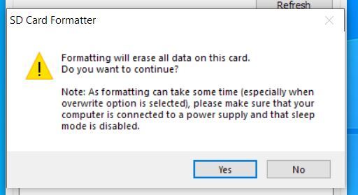
- Click “Format” to start formatting, and “Yes” on the warning dialog.
Here are the screenshots I took of the process:
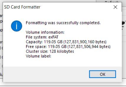
When you get the notification that the formatting was successfully, close all open windows.
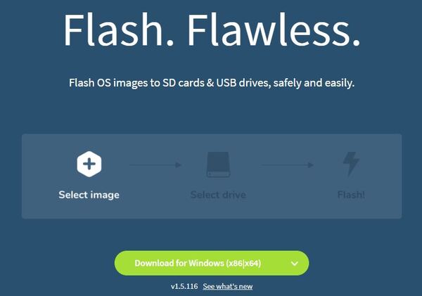
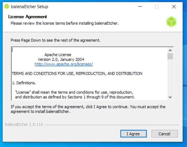
Now download, install, and launch Etcher.
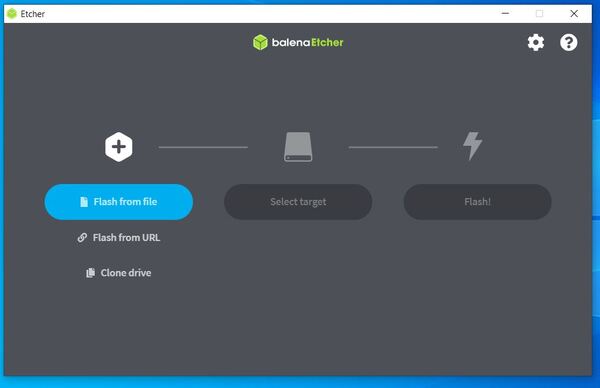
Click “Flash from file” and choose the zipped Nano Jetson image file you downloaded earlier.
Insert your microSD card if not already inserted.
Click “Select target” and choose the SD card’s drive. Remember mine is on the F drive.
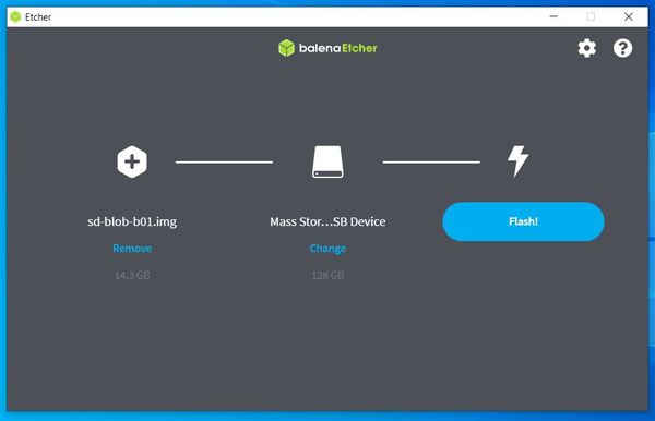
Click “Flash!” It will take Etcher a while to write and validate the image, so go do something else and come back.
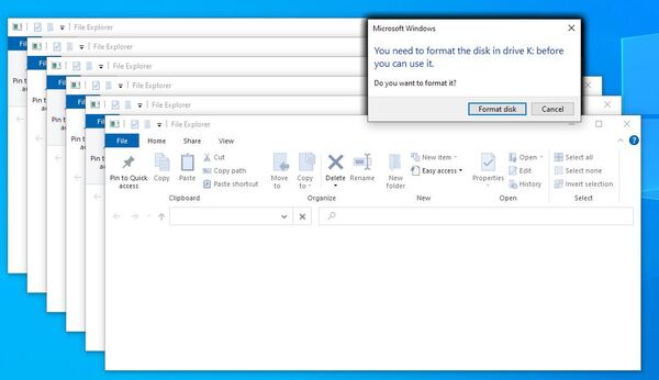
After Etcher finishes, Windows may let you know it doesn’t know how to read the SD Card. Just click Cancel all those screens and remove the microSD card.
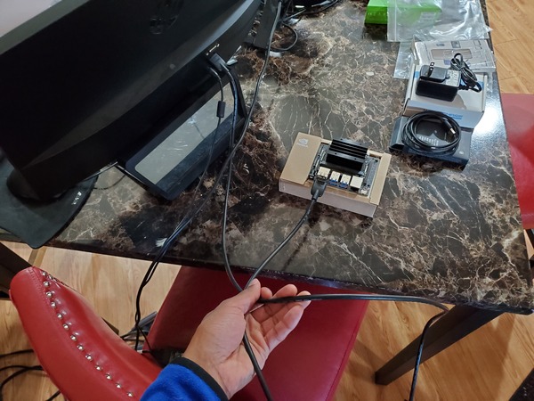
Setup and First Boot
Unfold the paper stand, and place the Nano Jetson inside the developer kit box.
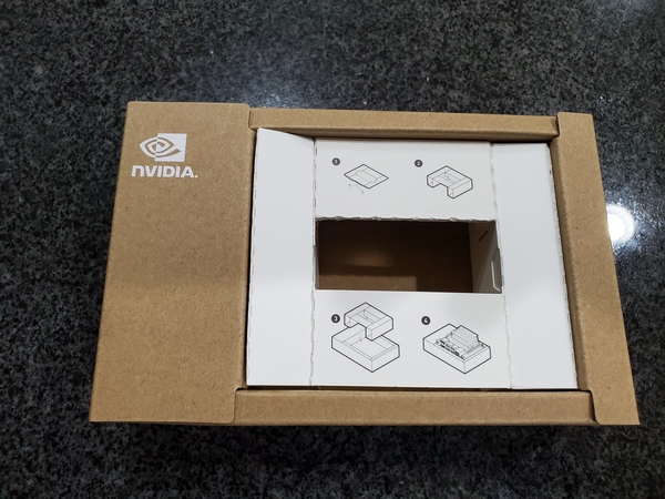
Set the developer kit on top of the paper stand.
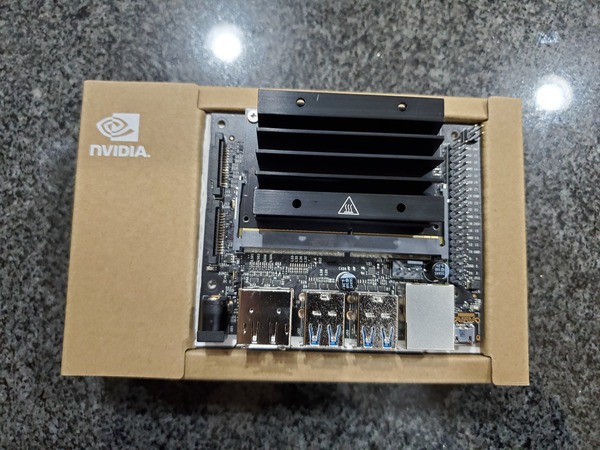
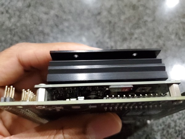
Insert the microSD card (with system image already written to it) into the slot on the underside of the Jetson Nano module.
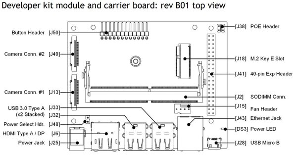
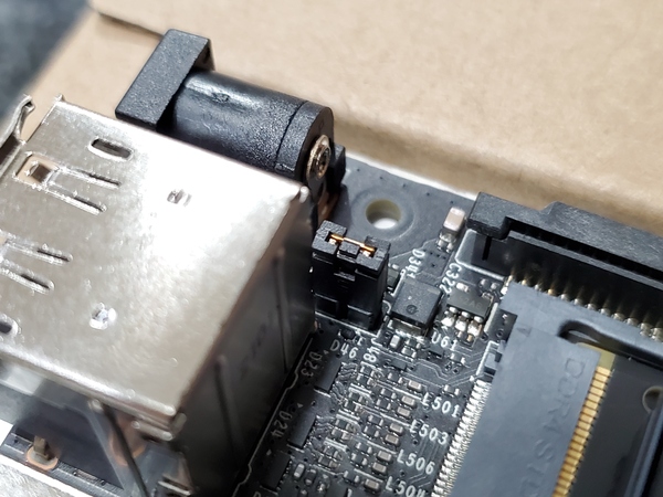
Make sure the jumper is pushed into the J48 Power Select Header pins.
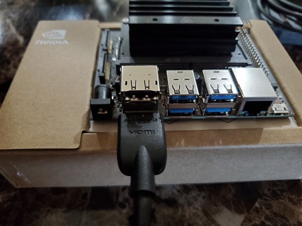
Connect the Jetson Nano into your monitor. I am using an HDMI cable to connect my monitor to my Jetson Nano. If you don’t have one, you can buy one off Amazon or any other electronic retailer.
Connect the Jetson Nano into your keyboard.
Connect the Jetson Nano into your mouse.
Grab the “Power Supply Applicable for Jetson Nano 5V/4A OD 5.5mm ID 2.1mm”.
Connect the power supply to the 5V/4A Power Jack. The developer kit will power on automatically.
Allow 1 minute for the developer kit to boot.
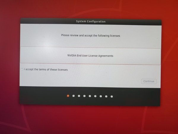
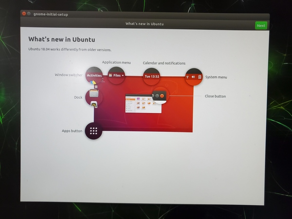
A green LED next to the Micro-USB connector will light as soon as the developer kit powers on. When you boot the first time, the developer kit will take you through some initial setup, including:
Review and accept NVIDIA Jetson software End User License Agreement.
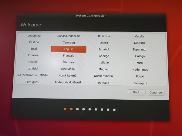
Select the system language.
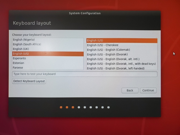
Select the keyboard layout.
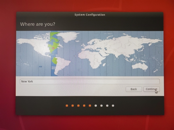
Select the time zone.
Create a username, password, and computer name. Be sure to select “Log in automatically.”
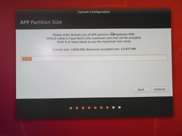
Select APP partition size. NVIDIA recommends to use the maximum size.
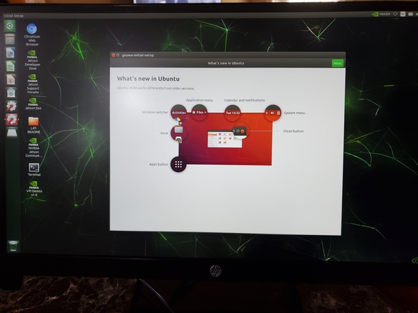
Here is the screen you should see now.
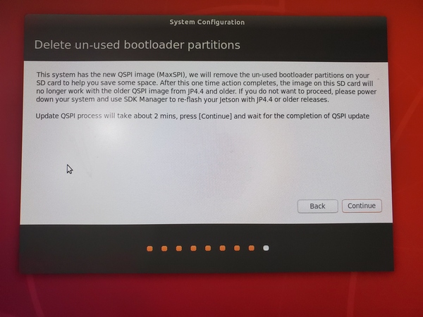
Update QSPI process and click Continue.
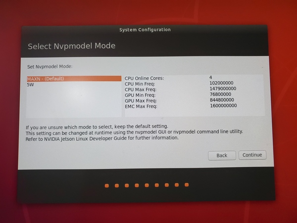
Keep the default setting for the Nvpmodel Mode, and click Continue.
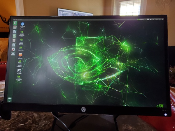
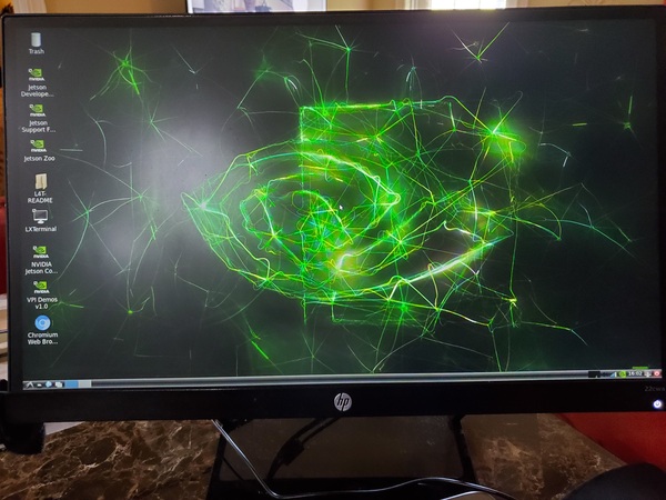
Your Nvidia will automatically reboot to the Ubuntu desktop.
Click the Terminal icon in the bottom-left.
Restart the computer again.
sudo reboot
Set Up WiFi
Grab your WiFi adapter.
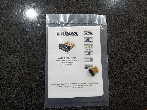
Plug it into one of the USB ports on the Jetson Nano.
To set up WiFi, you can use the following command in a terminal window (sudo nmtui), or follow the steps below.
Click the settings (gear) icon in the upper right corner of the desktop.
Click System Settings in the drop down menu.
Click the Network dialog in the dialog box.
Set up the network connection.
Reboot the computer.
sudo reboot
Your computer might pop up a Software Updater dialog. You can click Install Now.
Right click on the Desktop.
Open the Terminal.
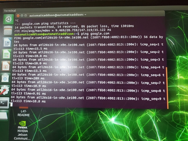
Check if your WiFi setup is fine.
ping google.com
Turn off the power save mode to get stability.
sudo iw dev wlan0 set power_save off
sudo reboot
Run Updates
Let’s update our package list and upgrade the software on the system.
Open the terminal, and type:
sudo apt-get update
sudo apt-get upgrade
Type Y and press Enter to upgrade everything.
Reboot the computer.
sudo reboot
Collect Information About Your Jetson Nano
Open a terminal window, and type the following command.
hostname -I
Make a note of your internal IP address.
Change the Power Supply Settings
If you are using the 5V/4A power supply like I am, open your terminal window, and type:
sudo nvpmodel -q
If you see the following, you are good to go.
NV Power Mode: MAXN
Otherwise, type the following command:
sudo nvpmodel -m 0
This command will give you high power performance. If you want to change it to low performance because you are using microUSB to power the Jetson Nano, here is the command:
sudo nvpmodel -m 1
Create a Swap File
Some of the applications I will use on my Jetson Nano require a lot of memory. To keep the Nano from crashing, we need to create a swap file.
See if your Nano already has swap space.
free -h
If you don’t have swap space, add a 4GB swap file.
sudo fallocate -l 4G /var/swapfile
sudo chmod 600 /var/swapfile
sudo mkswap /var/swapfile
sudo swapon /var/swapfile
sudo bash -c 'echo "/var/swapfile swap swap defaults 0 0" >> /etc/fstab'
Reboot your Nano.
sudo reboot
Once the Nano is done rebooting, see if you have swap space.
free -h
Connect to Your NVIDIA Jetson Nano Remotely From Your PC
Now I will show you everything you need to know to connect to your NVIDIA Jetson Nano desktop remotely from your own PC (on the same WiFi network) using an application called VNC Viewer.
Save RAM By Using the LXDE Desktop
First, let’s free up some RAM to keep our Nano from crashing.
Type the following command. Your computer will then reboot to a login screen.
$DESKTOP_SESSION
On the login screen, click the gear icon next to “Sign In”.
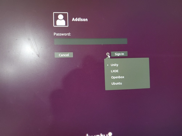
Scroll down, and select LXDE.
Type your password, and click Sign In.
LXDE is now your desktop environment.
Reboot.
sudo reboot
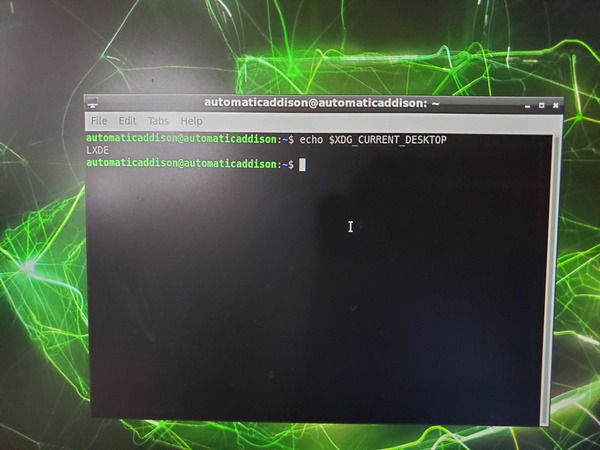
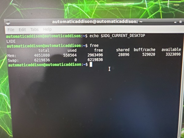
Open a terminal window in your Nano, and type the following command to see what desktop environment you’re using.
echo $XDG_CURRENT_DESKTOP
See how much free memory you have.
free
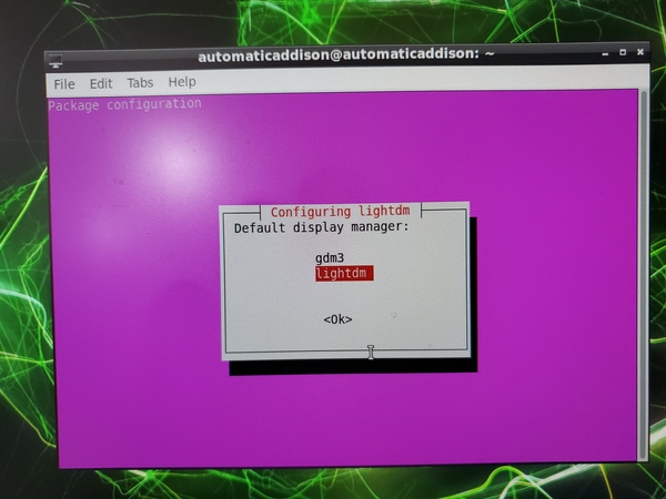
Now open a terminal window, and change the display manager from gdm3 (GNOME display manager) to lightdm.
sudo dpkg-reconfigure lightdm
You will see a window pop up.
Press Enter.
Next, select lightdm, and press Enter.
Reboot your computer.
sudo reboot
Open a new terminal window, and type:
free
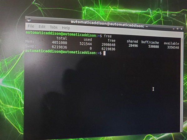
You can see that we now have less memory used.
Set Up the VNC Server
Now we need to set up the VNC server.
First, enable the VNC server to start each time you log in. Open a new terminal window, and type:
mkdir -p ~/.config/autostart
cp /usr/share/applications/vino-server.desktop ~/.config/autostart/.
Now, we need to configure the VNC server.
gsettings set org.gnome.Vino prompt-enabled false
gsettings set org.gnome.Vino require-encryption false
Set a password for the VNC server. Make sure you remember it.
# Replace thepassword with your desired password
gsettings set org.gnome.Vino authentication-methods "['vnc']"
gsettings set org.gnome.Vino vnc-password $(echo -n 'thepassword'|base64)
Shutdown your Jetson Nano.
sudo shutdown -h now
Once the Jetson Nano is OFF, unplug the 5V/4A power source.
Unplug your mouse, keyboard, and monitor from the Jetson Nano.
Plug the 5V/4A power source back into the Jetson Nano.
Install a Remote Desktop Software
Option 1 (Slowest): VNC Viewer on Your PC
To install VNC Viewer, I will follow these instructions that cover Windows, MacOs, and Linux.
If you’re using Windows, go to your PC, and download and install VNC Viewer.
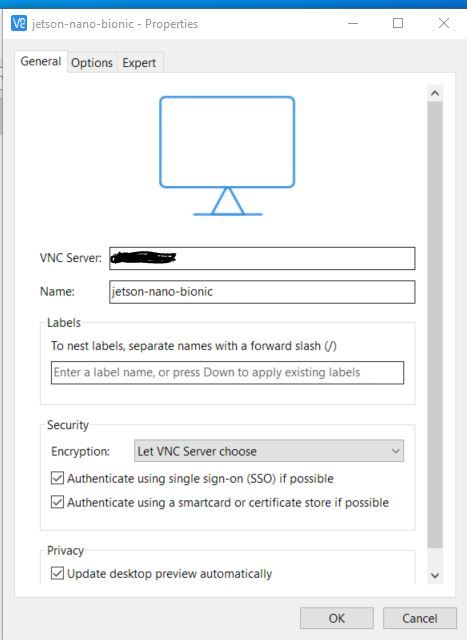
Launch the VNC viewer and type in the IP address of your Jetson Nano. You can also go to File -> New Connection
If you have configured the VNC server for authentication, provide the VNC password.
The remote desktop connection lag might be very strong.You change the desktop resolution by clicking in the bottom-left and going to Preference -> Monitor settings.
I’m not a huge fan of the remote desktop for the Jetson Nano. Raspberry Pi is far superior. Hopefully the guys at NVIDIA fix that in the future by building in WiFi to their boards.
Now, power OFF your Jetson Nano.
sudo shutdown -h now
Remove the power supply, and then plug it back in.
Option 2 (Fastest): Install NoMachine on Your PC
VNC Viewer was too slow for me on Windows, so I installed NoMachine. I will follow these instructions and these instructions.
Go to the NoMachine website and download the DEB package for ARMv8.
This folder will go to your Downloads folder. Move to that folder via the terminal.
cd Downloads
Install NoMachine with the ‘dpkg’ command. For example if you downloaded package ‘nomachine_7.4.1_1_arm64.deb’:
sudo dpkg -i nomachine_7.4.1_1_arm64.deb
Now click on the start menu in the bottom-left. Select NoMachine. NoMachine might be under the “Internet” option.
Make a note of the URL you can use to connect to your Jetson Nano.
Restart your Jetson Nano.
sudo shutdown -h now
Unplug the power supply from your Jetson Nano.
Plug the power supply into your Jetson Nano.
Now download the NoMachine software from your own PC (Windows, MacOs, or Linux).
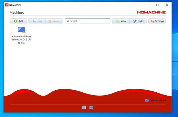
After you have downloaded it, launch the NoMachine application on your PC.
Double click on your Jetson Nano icon (i.e. Ubuntu 18.04).
Click Yes.
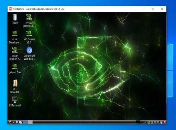
Type in the username and password for the Jetson Nano machine.
Click through the prompts, and you will see your Desktop appear.
Now, power OFF your Jetson Nano.
sudo shutdown -h now
Remove the power supply, and then plug it back in.
Install Putty (Optional)
Putty is a program that will enable us to connect to the Jetson Nano’s terminal only.
Go to putty.org and download the installer for your machine. I am using a 64-bit Windows computer so that is what I will select.
Follow the instructions to download Putty. Once you’ve finished, open up Putty. If you’re using Windows, you can usually find it in the Start Menu.
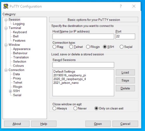
The first thing you will do is type in the IP address of your Jetson Nano.
Select the SSH radio button.
Click the Open button.
If you get a popup window, click “Yes” and then you will go to a black terminal window.
Type in the username and password of your Jetson Nano.
That’s it. You’re logged in to your Jetson Nano via the command line interface.
You are now good to go.
Next Steps
A lot of Jetson Nano projects involve heavy computation (e.g. deep learning and robotics), which can make the board heat up pretty quickly. I recommend buying and setting up your Jetson Nano with a cooling fan and case.
Whew! That was a lot of work setting up the NVIDIA Jetson Nano.
That’s it. Keep building!