In this tutorial, we will write a basic Python program for NVIDIA Jetson Nano.
Prerequisites
- You have already set up your NVIDIA Jetson Nano.
- This tutorial will be similar to my Python fundamentals for robotics tutorial.
Install Python
To install Python, open a new terminal window and type:
sudo apt-get install python python3
To find out where the Python interpreter is located, type this command.
which python
You should see:
/usr/bin/python
Install Gedit
Install gedit, a text editor that will enable us to write code in Python.
sudo apt-get install gedit
Install Pip
Let’s begin by installing pip. Pip is a tool that will help us manage software packages for Python.
Software packages are bundles of code written by someone else that are designed to solve a specific problem. Why write code to solve a specific problem from scratch, when someone else has already written code to solve that exact same problem? That is where software packages come into play. They prevent you from having to reinvent the wheel.
Open up a fresh Linux terminal window.
Type the following command to update the list of available packages that can be installed on your system.
sudo apt-get update
Type your password.
Upgrade all the packages. The -y flag in the following command is used to confirm to our computer that we want to upgrade all the packages.
sudo apt-get -y upgrade
Type the following command to check the version of Python you have installed.
python3 --version
My version is 3.6.9. Your version might be different. That’s fine.
Now, let’s install pip.
sudo apt-get install -y python3-pip
If at any point in the future you want to install a Python-related package using pip, you can use the following command:
pip3 install package_name
Create a Virtual Environment
In this section, we will set up a virtual environment. You can think of a virtual environment as an independent workspace with its own set of libraries, settings, packages, and programming language versions installed.
For example, you might have a project that needs to run using an older version of Python, like Python 2.7. You might have another project that requires Python 3.8. Setting up separate virtual environments for each project will make sure that the projects stay isolated from one another.
Let’s install the virtual environment package.
sudo apt-get install -y python3-venv
With the software installed, we can now create the virtual environment using the following command. The dot(.) in front of py3venv makes the directory a hidden directory (the dot is optional):
python3 -m venv .py3venv
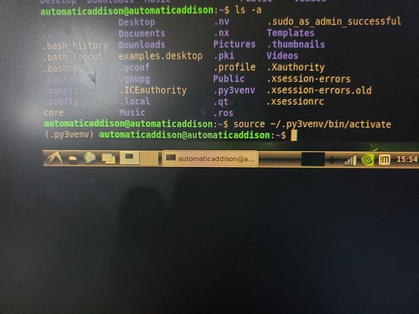
Type the following command to get a list of all the directories. You should see the .py3venv folder there.
ls -a
List all the contents inside the .py3venv folder.
ls .py3venv/
Now that the virtual environment has been created, we can activate it using the following command:
source ~/.py3venv/bin/activate
Look what happened. There is a prefix on the current line that has the name of the virtual environment we created. This prefix means that the .py3venv virtual environment is currently active.
When a virtual environment is active that means that when we create software programs here in Python, these programs will use the settings and packages of just this virtual environment.
Keep your terminal window open. We’re not ready to close it just yet. Move on to the next section so that we can write our first program in Python.
Write a “Hello World” Program
Let’s write a program that does nothing but print “Hello Automatic Addison” (i.e. my version of a “Hello World” program) to the screen.
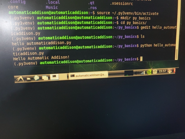
Create a new folder.
mkdir py_basics
Move to that folder.
cd py_basics
Open a new Python program.
gedit hello_automaticaddison.py
Type the following code in there:
#!/usr/bin/env python
print("Hello Automatic Addison!")
Save the file, and close it.
See if your file is in there.
ls
Run the program.
python hello_automaticaddison.py
Deactivate the virtual environment.
deactivate
That’s it. Keep building!