In this tutorial, I will show you how to create and implement a complex action using ROS 2 Galactic, the latest version of ROS 2. The official tutorial (with a basic example) is here, and other examples are here. I will walk through all the steps below.
The action we will create in this tutorial can be used to simulate a mobile robot connecting to a battery charging dock.
Prerequisites
- ROS 2 Foxy Fitzroy installed on Ubuntu Linux 20.04 or newer. I am using ROS 2 Galactic, which is the latest version of ROS 2 as of the date of this post.
- You have already created a ROS 2 workspace. The name of our workspace is “dev_ws”, which stands for “development workspace.”
- You have Python 3.7 or higher.
You can find the files for this post here on my Google Drive.
QuickStart
Let’s take a look at the ROS 2 demo repository so we can examine the sample action they created in their official tutorial.
Open a new terminal window, and clone the action_tutorials repository from GitHub.
cd ~dev_ws/src
git clone https://github.com/ros2/demos.git
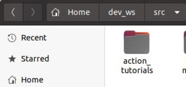
You only need the action_tutorials folder (which is inside the folder named ‘demos’), so cut and paste that folder into the ~/dev_ws/src folder using your File Explorer. You can then delete the demos folder.
Once you have your ~dev_ws/src/action_tutorials folder, you need to build it. Open a terminal window, and type:
cd ..
colcon build
You now have three new packages:
- action_tutorials_cpp
- action_tutorials_py
- action_tutorials_interfaces.
First, we will work with the action_tutorials_interfaces tutorial package.
To see if everything is working, let’s take a look at the definition of the action created in the official tutorial.
Open a new terminal window, and type:
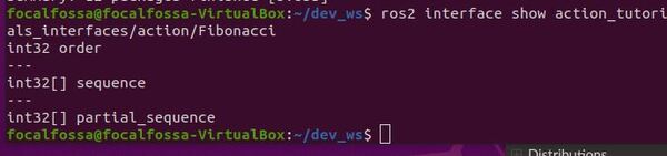
ros2 interface show action_tutorials_interfaces/action/Fibonacci
Here is the output you should see:
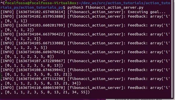
Now launch the action server.
cd ~/dev_ws/src/action_tutorials/action_tutorials_py/action_tutorials_py
python3 fibonacci_action_server.py
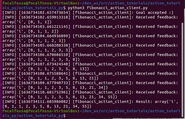
In another terminal, send a goal to the action server.
python3 fibonacci_action_client.py
Here is the output:
Define the ConnectToChargingDock Action
Now that we see everything is working properly, let’s define a new action. The action we will create will be used to connect a mobile robot to a charging dock.
Open a terminal window, and move to your package.
cd ~/dev_ws/src/action_tutorials/action_tutorials_interfaces/action
Create a file called ConnectToChargingDock.action.
gedit ConnectToChargingDock.action
Add this code.
sensor_msgs/BatteryState desired_battery_state
---
sensor_msgs/BatteryState final_battery_state
---
sensor_msgs/BatteryState current_battery_state
Save the file and close it.
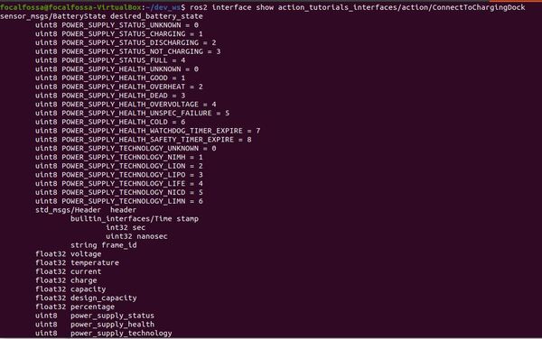
You can see the action definition has three sections:
- Request: desired_battery_state
- Result: final_battery_state
- Feedback: current_battery_state
Build the Action
Go to your CMakeLists.txt file.
cd ~/dev_ws/src/action_tutorials/action_tutorials_interfaces
gedit CMakeLists.txt
Make sure your CMakeLists.txt file has the following lines added in the proper locations.
find_package(sensor_msgs REQUIRED)
find_package(std_msgs REQUIRED)

rosidl_generate_interfaces(${PROJECT_NAME}
  "action/Fibonacci.action"
  "action/ConnectToChargingDock.action"
  DEPENDENCIES sensor_msgs std_msgs
)
Save the CMakeLists.txt file, and close it.
Now edit your package.xml file.
cd ~/dev_ws/src/action_tutorials/action_tutorials_interfaces
gedit package.xml
Add the dependencies.
<depend>sensor_msgs</depend>
<depend>std_msgs</depend>
Here is my full package.xml file.
Build the package.
cd ~/dev_ws/
colcon build
Let’s check to see if the action was built properly.
Open another terminal window, and type (all of this is a single command):
ros2 interface show action_tutorials_interfaces/action/ConnectToChargingDock
Here is the output:
Write the Action Server
Now let’s create our action server. We will create an action server that will send velocity commands to the /cmd_vel topic until the power_supply_status of the battery state switches from 3 (i.e. not charging) to 1 (i.e. charging).
Open a terminal window and type:
cd ~/dev_ws/src/action_tutorials/action_tutorials_py/action_tutorials_py
Open a file called connect_to_charging_dock_action_server.py.
gedit connect_to_charging_dock_action_server.py
Add the following code:
#!/usr/bin/env python3
"""
Description:
  Action Server to connect to a battery charging dock.
  Action is successful when the power_supply_status goes from
  NOT_CHARGING(i.e. 3) to CHARGING(i.e. 1)
-------
Subscription Topics:
  Current battery state
  /battery_status – sensor_msgs/BatteryState
-------
Publishing Topics:
  Velocity command to navigate to the charging dock.
  /cmd_vel - geometry_msgs/Twist
-------
Author: Addison Sears-Collins
Website: AutomaticAddison.com
Date: November 12, 2021
"""
import time

# Import our action definition
from action_tutorials_interfaces.action import ConnectToChargingDock

# ROS Client Library for Python
import rclpy

# ActionServer library for ROS 2 Python
from rclpy.action import ActionServer

# Enables publishers, subscribers, and action servers to be in a single node
from rclpy.executors import MultiThreadedExecutor

# Handles the creation of nodes
from rclpy.node import Node

# Handle Twist messages, linear and angular velocity
from geometry_msgs.msg import Twist

# Handles BatteryState message
from sensor_msgs.msg import BatteryState

# Holds the current state of the battery
this_battery_state = BatteryState()

class ConnectToChargingDockActionServer(Node):
  """
  Create a ConnectToChargingDockActionServer class,
  which is a subclass of the Node class.
  """
  def __init__(self):

    # Initialize the class using the constructor
    super().__init__('connect_to_charging_dock_action_server')

    # Instantiate a new action server
    # self, type of action, action name, callback function for executing goals
    self._action_server = ActionServer(
      self,
      ConnectToChargingDock,
      'connect_to_charging_dock',
      self.execute_callback)

    # Create a publisher
    # This node publishes the desired linear and angular velocity of the robot
    self.publisher_cmd_vel = self.create_publisher(
      Twist,
      '/cmd_vel',
      10)

    # Declare velocities
    self.linear_velocity = 0.0
    self.angular_velocity = 0.15

  def execute_callback(self, goal_handle):
    """
    Action server callback to execute accepted goals.
    """
    self.get_logger().info('Executing goal...')

    # Interim feedback
    feedback_msg = ConnectToChargingDock.Feedback()
    feedback_msg.current_battery_state = this_battery_state

    # While the battery is not charging
    while this_battery_state.power_supply_status != 1:

      # Publish the current battery state
      feedback_msg.current_battery_state = this_battery_state
      self.get_logger().info('NOT CHARGING...')
      goal_handle.publish_feedback(feedback_msg)

      # Send the velocity command to the robot by publishing to the topic
      cmd_vel_msg = Twist()
      cmd_vel_msg.linear.x = self.linear_velocity
      cmd_vel_msg.angular.z = self.angular_velocity
      self.publisher_cmd_vel.publish(cmd_vel_msg)

      time.sleep(0.1)

    # Stop the robot
    cmd_vel_msg = Twist()
    cmd_vel_msg.linear.x = 0.0
    cmd_vel_msg.angular.z = 0.0
    self.publisher_cmd_vel.publish(cmd_vel_msg)

    # Update feedback
    feedback_msg.current_battery_state = this_battery_state
    goal_handle.publish_feedback(feedback_msg)

    # Indicate the goal was successful
    goal_handle.succeed()
    self.get_logger().info('CHARGING...')
    self.get_logger().info('Successfully connected to the charging dock!')

    # Create a result message of the action type
    result = ConnectToChargingDock.Result()

    # Update the final battery state
    result.final_battery_state = feedback_msg.current_battery_state

    return result

class BatteryStateSubscriber(Node):
    """
    Subscriber node to the current battery state
    """
    def __init__(self):

      # Initialize the class using the constructor
      super().__init__('battery_state_subscriber')

      # Create a subscriber
      # This node subscribes to messages of type
      # sensor_msgs/BatteryState
      self.subscription_battery_state = self.create_subscription(
        BatteryState,
        '/battery_status',
        self.get_battery_state,
        10)

    def get_battery_state(self, msg):
      """
      Update the current battery state.
      """
      global this_battery_state
      this_battery_state = msg

def main(args=None):
  """
  Entry point for the program.
  """

  # Initialize the rclpy library
  rclpy.init(args=args)

  try:

    # Create the Action Server node
    connect_to_charging_dock_action_server = ConnectToChargingDockActionServer()

    # Create the Battery State subscriber node
    battery_state_subscriber = BatteryStateSubscriber()

    # Set up mulithreading
    executor = MultiThreadedExecutor(num_threads=4)
    executor.add_node(connect_to_charging_dock_action_server)
    executor.add_node(battery_state_subscriber)

    try:
      # Spin the nodes to execute the callbacks
      executor.spin()
    finally:
      # Shutdown the nodes
      executor.shutdown()
      connect_to_charging_dock_action_server.destroy_node()
      battery_state_subscriber.destroy_node()

  finally:
    # Shutdown
    rclpy.shutdown()

if __name__ == '__main__':
    main()
Save the code and close it.
Open your package.xml file.
cd ~/dev_ws/src/action_tutorials/action_tutorials_py/
gedit package.xml
Add the dependencies:
<exec_depend>geometry_msgs</exec_depend>
<exec_depend>sensor_msgs</exec_depend>
<exec_depend>std_msgs</exec_depend>
Save the file and close it.
cd ~/dev_ws/src/action_tutorials/action_tutorials_py/
Open your setup.py file.
Add the following line inside the entry_points block.
'connect_to_charging_dock_server = action_tutorials_py.connect_to_charging_dock_action_server:main',Save the file and close it.
Run the node.
cd ~/dev_ws
colcon build
Run the Action Server
Now let’s run a simulation. First, let’s assume the battery voltage on our robot is below 25%, and the robot is currently positioned at a location just in front of the charging dock. Our robot is running on a 9V battery, and we want the robot to connect to the charging dock so the power supply status switches from NOT CHARGING to CHARGING.
To simulate a ‘low battery’, we publish a message to the /battery_status topic.
Open a terminal window, and type:
ros2 topic pub /battery_status sensor_msgs/BatteryState '{voltage: 2.16, percentage: 0.24, power_supply_status: 3}'
The above command means the battery voltage is 2.16V (24% of 9V), and the battery is NOT CHARGING because the power_supply_status variable is 3.
Now, let’s launch the action server. Open a new terminal window, and type:
ros2 run action_tutorials_py connect_to_charging_dock_server
Open a new terminal window, and send the action server a goal.
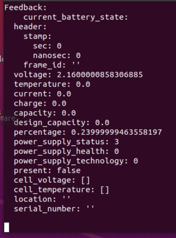
ros2 action send_goal --feedback connect_to_charging_dock action_tutorials_interfaces/action/ConnectToChargingDock "desired_battery_state: {voltage: 2.16, percentage: 0.24, power_supply_status: 1}}"
The goal above means we want the power_supply_status to be 1 (i.e. CHARGING). Remember, it is currently 3 (NOT CHARGING).
You should see this feedback:
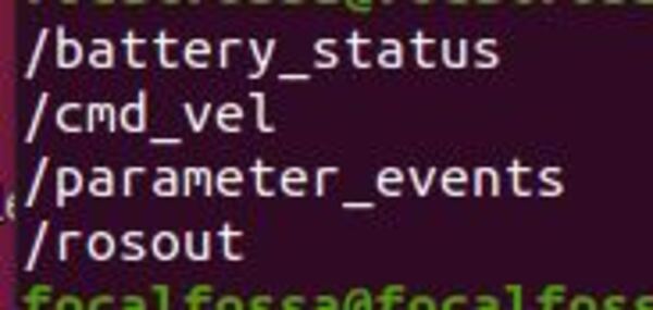
Let’s see what is going on behind the scenes. Open a new terminal window, and check out the list of topics:
ros2 topic list
To see the node graphs, type:
rqt_graph
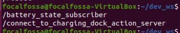
To see the active nodes, type:
ros2 node list
To see the available actions, type:
ros2 action list
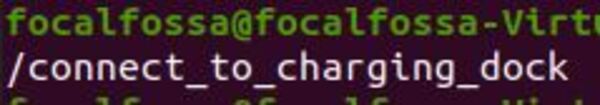
You can see full information about the node, by typing:
ros2 node info /connect_to_charging_dock_action_server
You can see more information about the action by typing:
ros2 action info /connect_to_charging_dock
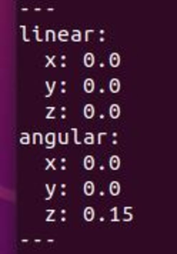
Now type:
ros2 topic echo /cmd_vel
You can see that our action server is publishing velocity commands to the /cmd_vel topic. Right now, I have the robot doing a continuous spin at 0.15 radians per second. In a real-world application, you will want to add code to the action server to read from infrared sensors or an ARTag in order to send the appropriate velocity commands.
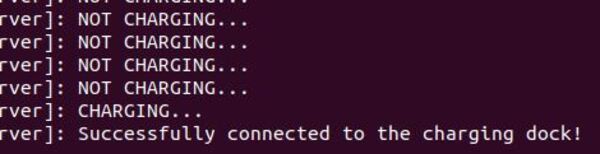
Finally, let’s assume our robot has connected to the charging dock. To make the power_supply_status switch from 3 (NOT CHARGING) to 1 (CHARGING), stop the /battery_status publisher by going back to that terminal window, and typing:
CTRL + C
Then open a terminal window, and type:
ros2 topic pub /battery_status sensor_msgs/BatteryState '{voltage: 2.16, percentage: 0.24, power_supply_status: 1}'
Here is the output on the action server window:
The action client window has the following output:
Write the Action Client
Now that we have written the action server, let’s write the action client. The official tutorial is here.
The action client’s job is to send a goal to the action server. In the previous section, we used a terminal command to do this, but now we will use code.
Open a terminal window and type:
cd ~/dev_ws/src/action_tutorials/action_tutorials_py/action_tutorials_py
Open a file called connect_to_charging_dock_action_client.py.
gedit connect_to_charging_dock_action_client.py
Add the following code:
#!/usr/bin/env python3
"""
Description:
  Action Client to connect to a battery charging dock.
  Action is successful when the power_supply_status goes from
  NOT_CHARGING(i.e. 3) to CHARGING(i.e. 1)
-------
Author: Addison Sears-Collins
Website: AutomaticAddison.com
Date: November 13, 2021
"""
# Import our action definition
from action_tutorials_interfaces.action import ConnectToChargingDock

# ROS Client Library for Python
import rclpy

# ActionClient library for ROS 2 Python
from rclpy.action import ActionClient

# Handles the creation of nodes
from rclpy.node import Node

# Handles BatteryState message
from sensor_msgs.msg import BatteryState

class ConnectToChargingDockActionClient(Node):
  """
  Create a ConnectToChargingDockActionClient class,
  which is a subclass of the Node class.
  """
  def __init__(self):

    # Initialize the class using the constructor
    super().__init__('connect_to_charging_dock_action_client')

    # Instantiate a new action client
    # self, type of action, action name
    self._action_client = ActionClient(
      self,
      ConnectToChargingDock,
      'connect_to_charging_dock')

  def send_goal(self, desired_battery_state):
    """
    Action client to send the goal
    """
    # Set the goal message
    goal_msg = ConnectToChargingDock.Goal()
    goal_msg.desired_battery_state = desired_battery_state

    # Wait for the Action Server to launch
    self._action_client.wait_for_server()

    # Register a callback for when the future is complete
    self._send_goal_future = self._action_client.send_goal_async(goal_msg, feedback_callback=self.feedback_callback)
    self._send_goal_future.add_done_callback(self.goal_response_callback)

  def goal_response_callback(self, future):
    """
    Get the goal_handle
    """
    goal_handle = future.result()
    if not goal_handle.accepted:
      self.get_logger().info('Goal rejected...')
      return

    self.get_logger().info('Goal accepted...')

    self._get_result_future = goal_handle.get_result_async()
    self._get_result_future.add_done_callback(self.get_result_callback)

  def get_result_callback(self, future):
    """
    Gets the result
    """
    result = future.result().result
    self.get_logger().info('Result (1 = CHARGING, 3 = NOT CHARGING): {0}'.format(
      result.final_battery_state.power_supply_status))
    rclpy.shutdown()

  def feedback_callback(self, feedback_msg):
    feedback = feedback_msg.feedback
    self.get_logger().info(
      'Received feedback (1 = CHARGING, 3 = NOT CHARGING): {0}'.format(
      feedback.current_battery_state.power_supply_status))

def main(args=None):
  """
  Entry point for the program.
  """

  # Initialize the rclpy library
  rclpy.init(args=args)

  # Create the goal message
  desired_battery_state = BatteryState()
  desired_battery_state.voltage = 2.16
  desired_battery_state.percentage = 0.24
  desired_battery_state.power_supply_status = 1

  # Create the Action Client node
  action_client = ConnectToChargingDockActionClient()

  # Send the goal
  action_client.send_goal(desired_battery_state)

  # Spin to execute callbacks
  rclpy.spin(action_client)

if __name__ == '__main__':
    main()
Save the code and close it.
Now type:
cd ~/dev_ws/src/action_tutorials/action_tutorials_py/
Open your setup.py file.
Add the following line inside the entry_points block.
'connect_to_charging_dock_client = action_tutorials_py.connect_to_charging_dock_action_client:main',
Save the file and close it.
Run the node.
cd ~/dev_ws
colcon build
Run the Action Server and Client Together
To simulate a ‘low battery’, we publish a message to the /battery_status topic.
Open a terminal window, and type:
ros2 topic pub /battery_status sensor_msgs/BatteryState '{voltage: 2.16, percentage: 0.24, power_supply_status: 3}'
Now, let’s launch the action server. Open a new terminal window, and type:
ros2 run action_tutorials_py connect_to_charging_dock_server
Open a new terminal window, and send the action server a goal using the action client.
ros2 run action_tutorials_py connect_to_charging_dock_client
Stop the /battery_status publisher by going back to that terminal window, and typing:
CTRL + C
Then open a terminal window, and type:
ros2 topic pub /battery_status sensor_msgs/BatteryState '{voltage: 2.16, percentage: 0.24, power_supply_status: 1}'
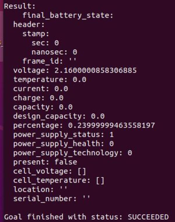
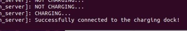
Here is the output on the action server window:
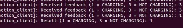
The action client window has the following output:
There you have it. The code in this tutorial can be used as a template for autonomous docking at a charging station.
Keep building!