Real-Time Object Tracking Using OpenCV and a Webcam

In this tutorial, we will create a program to track a moving object in real-time using the built-in webcam of a laptop computer. We will use Python and the OpenCV computer vision library for the code.
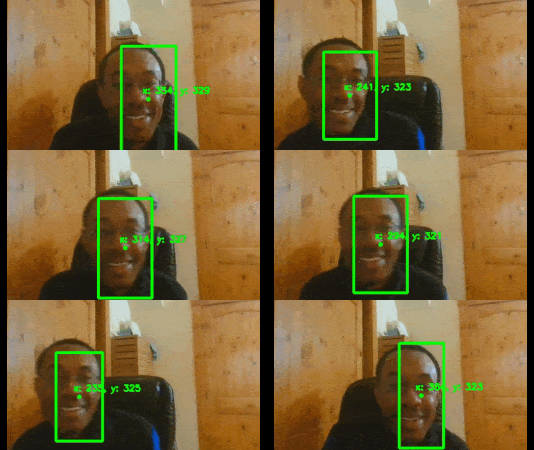
real-time-object-tracking-webcam-opencv

A real-world application of this is in robotics. Imagine you have a robot arm that needs to continuously pick up moving items from a conveyor belt inside a warehouse. In order for the robot to pick up an object it needs to know the exact coordinates of the object. The program we will create below will give you the basic building block to do just that. It will locate the coordinates of the center of the moving object (often called the “centroid“) in real-time using an ordinary webcam.

Let’s get started!

Prerequisites

  • Python 3.7 or higher

Requirements

Using real-time streaming video from your built-in webcam, create a program that:

  • Draws a bounding box around a moving object
  • Calculates the coordinates of the centroid of the object
  • Tracks the centroid of the object

Directions

Open up your favorite IDE or code editor.

Make sure you have the OpenCV and Numpy libraries installed. There are a number of ways to install both libraries. The most common way is to use pip, which is the standard package manager for Python.

pip install opencv-python
pip install numpy

Copy and paste the code below. This is all you need to run the program.

I put detailed comments inside the code so that you know what is going on. The technique used here is background subtraction, one of the most common ways to detect moving objects in a video stream:

#!/usr/bin/env python

'''
Welcome to the Object Tracking Program!

Using real-time streaming video from your built-in webcam, this program:
  - Creates a bounding box around a moving object
  - Calculates the coordinates of the centroid of the object
  - Tracks the centroid of the object

Author:
  - Addison Sears-Collins
  - https://automaticaddison.com
'''

from __future__ import print_function # Python 2/3 compatibility
import cv2 # Import the OpenCV library
import numpy as np # Import Numpy library

# Project: Object Tracking
# Author: Addison Sears-Collins 
# Website: https://automaticaddison.com
# Date created: 06/13/2020
# Python version: 3.7

def main():
    """
    Main method of the program.
    """

    # Create a VideoCapture object
    cap = cv2.VideoCapture(0)

    # Create the background subtractor object
    # Use the last 700 video frames to build the background
    back_sub = cv2.createBackgroundSubtractorMOG2(history=700, 
        varThreshold=25, detectShadows=True)

    # Create kernel for morphological operation
    # You can tweak the dimensions of the kernel
    # e.g. instead of 20,20 you can try 30,30.
    kernel = np.ones((20,20),np.uint8)

    while(True):

        # Capture frame-by-frame
        # This method returns True/False as well
        # as the video frame.
        ret, frame = cap.read()

        # Use every frame to calculate the foreground mask and update
        # the background
        fg_mask = back_sub.apply(frame)

        # Close dark gaps in foreground object using closing
        fg_mask = cv2.morphologyEx(fg_mask, cv2.MORPH_CLOSE, kernel)

        # Remove salt and pepper noise with a median filter
        fg_mask = cv2.medianBlur(fg_mask, 5) 
        
        # Threshold the image to make it either black or white
        _, fg_mask = cv2.threshold(fg_mask,127,255,cv2.THRESH_BINARY)

        # Find the index of the largest contour and draw bounding box
        fg_mask_bb = fg_mask
        contours, hierarchy = cv2.findContours(fg_mask_bb,cv2.RETR_TREE,cv2.CHAIN_APPROX_SIMPLE)[-2:]
        areas = [cv2.contourArea(c) for c in contours]

        # If there are no countours
        if len(areas) < 1:

            # Display the resulting frame
            cv2.imshow('frame',frame)

            # If "q" is pressed on the keyboard, 
            # exit this loop
            if cv2.waitKey(1) & 0xFF == ord('q'):
                break

            # Go to the top of the while loop
            continue

        else:
            # Find the largest moving object in the image
            max_index = np.argmax(areas)

        # Draw the bounding box
        cnt = contours[max_index]
        x,y,w,h = cv2.boundingRect(cnt)
        cv2.rectangle(frame,(x,y),(x+w,y+h),(0,255,0),3)

        # Draw circle in the center of the bounding box
        x2 = x + int(w/2)
        y2 = y + int(h/2)
        cv2.circle(frame,(x2,y2),4,(0,255,0),-1)

        # Print the centroid coordinates (we'll use the center of the
        # bounding box) on the image
        text = "x: " + str(x2) + ", y: " + str(y2)
        cv2.putText(frame, text, (x2 - 10, y2 - 10),
			cv2.FONT_HERSHEY_SIMPLEX, 0.5, (0, 255, 0), 2)
        
        # Display the resulting frame
        cv2.imshow('frame',frame)

        # If "q" is pressed on the keyboard, 
        # exit this loop
        if cv2.waitKey(1) & 0xFF == ord('q'):
            break

    # Close down the video stream
    cap.release()
    cv2.destroyAllWindows()

if __name__ == '__main__':
    print(__doc__)
    main()

How to Do Histogram Matching Using OpenCV

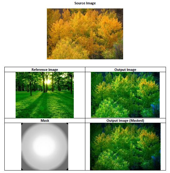
In this tutorial, you will learn how to do histogram matching using OpenCV. Histogram matching (also known as histogram specification), is the transformation of an image so that its histogram matches the histogram of an image of your choice (we’ll call this image of your choice the “reference image”).

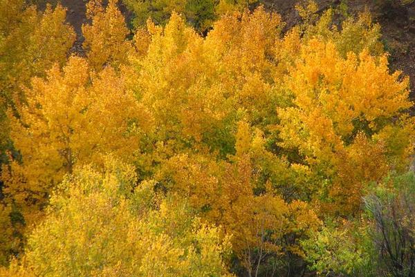
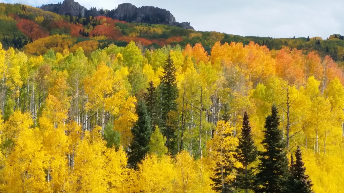
For example, consider this image below.

aspens_in_fall

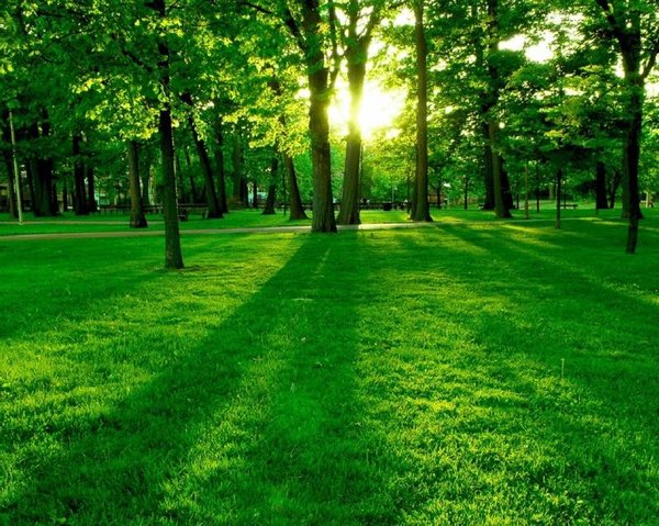
We want the image above to match the histogram of the reference image below.

forest-resized

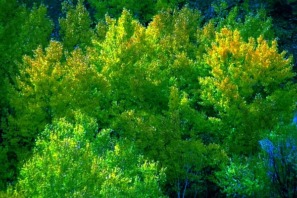
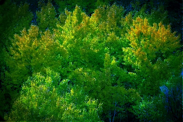
After performing histogram matching, the output image needs to look like this:

aspens_in_fall_forest_output

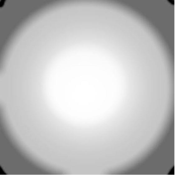
Then, to make things interesting, we want to use this mask to mask the output image.

mask
Mask
aspens_in_fall_forest_output_masked
Masked output image

You Will Need

Directions

Below is the source code for the program that makes everything happen. Make sure you copy and paste this code into a single Python file (mine is named histogram_matching.py). Then put that file, as well as your source, reference, and mask images all in the same directory (or folder) in your computer. Once you have done that, run the code using the following command (note: mask image is optional):

python histogram_matching.py <source_image> <ref_image> [<mask_image>]

For example (put this command all on one line):

python histogram_matching.py aspens_in_fall.jpg forest_resized.jpg mask.jpg

Source Code

#!/usr/bin/env python

'''
Welcome to the Histogram Matching Program!

Given a source image and a reference image, this program
returns a modified version of the source image that matches
the histogram of the reference image.

Image Requirements:
  - Source image must be color.
  - Reference image must be color.
  - The sizes of the source image and reference image do not
    have to be the same.
  - The program supports an optional third image (mask) as
    an argument.
  - When the mask image is provided, it will be rescaled to
    be the same size as the source image, and the resulting
    matched image will be masked by the mask image.

Usage:
  python histogram_matching.py <source_image> <ref_image> [<mask_image>]
'''

# Python 2/3 compatibility
from __future__ import print_function

import cv2 # Import the OpenCV library
import numpy as np # Import Numpy library
import matplotlib.pyplot as plt # Import matplotlib functionality
import sys # Enables the passing of arguments

# Project: Histogram Matching Using OpenCV
# Author: Addison Sears-Collins
# Date created: 9/27/2019
# Python version: 3.7

# Define the file name of the images
SOURCE_IMAGE = "aspens_in_fall.jpg"
REFERENCE_IMAGE = "forest_resized.jpg"
MASK_IMAGE = "mask.jpg"
OUTPUT_IMAGE = "aspens_in_fall_forest_output"
OUTPUT_MASKED_IMAGE = "aspens_in_fall_forest_output_masked.jpg"

def calculate_cdf(histogram):
    """
    This method calculates the cumulative distribution function
    :param array histogram: The values of the histogram
    :return: normalized_cdf: The normalized cumulative distribution function
    :rtype: array
    """
    # Get the cumulative sum of the elements
    cdf = histogram.cumsum()

    # Normalize the cdf
    normalized_cdf = cdf / float(cdf.max())

    return normalized_cdf

def calculate_lookup(src_cdf, ref_cdf):
    """
    This method creates the lookup table
    :param array src_cdf: The cdf for the source image
    :param array ref_cdf: The cdf for the reference image
    :return: lookup_table: The lookup table
    :rtype: array
    """
    lookup_table = np.zeros(256)
    lookup_val = 0
    for src_pixel_val in range(len(src_cdf)):
        lookup_val
        for ref_pixel_val in range(len(ref_cdf)):
            if ref_cdf[ref_pixel_val] >= src_cdf[src_pixel_val]:
                lookup_val = ref_pixel_val
                break
        lookup_table[src_pixel_val] = lookup_val
    return lookup_table

def match_histograms(src_image, ref_image):
    """
    This method matches the source image histogram to the
    reference signal
    :param image src_image: The original source image
    :param image  ref_image: The reference image
    :return: image_after_matching
    :rtype: image (array)
    """
    # Split the images into the different color channels
    # b means blue, g means green and r means red
    src_b, src_g, src_r = cv2.split(src_image)
    ref_b, ref_g, ref_r = cv2.split(ref_image)

    # Compute the b, g, and r histograms separately
    # The flatten() Numpy method returns a copy of the array c
    # collapsed into one dimension.
    src_hist_blue, bin_0 = np.histogram(src_b.flatten(), 256, [0,256])
    src_hist_green, bin_1 = np.histogram(src_g.flatten(), 256, [0,256])
    src_hist_red, bin_2 = np.histogram(src_r.flatten(), 256, [0,256])    
    ref_hist_blue, bin_3 = np.histogram(ref_b.flatten(), 256, [0,256])    
    ref_hist_green, bin_4 = np.histogram(ref_g.flatten(), 256, [0,256])
    ref_hist_red, bin_5 = np.histogram(ref_r.flatten(), 256, [0,256])

    # Compute the normalized cdf for the source and reference image
    src_cdf_blue = calculate_cdf(src_hist_blue)
    src_cdf_green = calculate_cdf(src_hist_green)
    src_cdf_red = calculate_cdf(src_hist_red)
    ref_cdf_blue = calculate_cdf(ref_hist_blue)
    ref_cdf_green = calculate_cdf(ref_hist_green)
    ref_cdf_red = calculate_cdf(ref_hist_red)

    # Make a separate lookup table for each color
    blue_lookup_table = calculate_lookup(src_cdf_blue, ref_cdf_blue)
    green_lookup_table = calculate_lookup(src_cdf_green, ref_cdf_green)
    red_lookup_table = calculate_lookup(src_cdf_red, ref_cdf_red)

    # Use the lookup function to transform the colors of the original
    # source image
    blue_after_transform = cv2.LUT(src_b, blue_lookup_table)
    green_after_transform = cv2.LUT(src_g, green_lookup_table)
    red_after_transform = cv2.LUT(src_r, red_lookup_table)

    # Put the image back together
    image_after_matching = cv2.merge([
        blue_after_transform, green_after_transform, red_after_transform])
    image_after_matching = cv2.convertScaleAbs(image_after_matching)

    return image_after_matching

def mask_image(image, mask):
    """
    This method overlays a mask on top of an image
    :param image image: The color image that you want to mask
    :param image mask: The mask
    :return: masked_image
    :rtype: image (array)
    """

    # Split the colors into the different color channels
    blue_color, green_color, red_color = cv2.split(image)

    # Resize the mask to be the same size as the source image
    resized_mask = cv2.resize(
        mask, (image.shape[1], image.shape[0]), cv2.INTER_NEAREST)

    # Normalize the mask
    normalized_resized_mask = resized_mask / float(255)

    # Scale the color values
    blue_color = blue_color * normalized_resized_mask
    blue_color = blue_color.astype(int)
    green_color = green_color * normalized_resized_mask
    green_color = green_color.astype(int)
    red_color = red_color * normalized_resized_mask
    red_color = red_color.astype(int)

    # Put the image back together again
    merged_image = cv2.merge([blue_color, green_color, red_color])
    masked_image = cv2.convertScaleAbs(merged_image)
    return masked_image

def main():
    """
    Main method of the program.
    """
    start_the_program = input("Press ENTER to perform histogram matching...") 

    # A flag to indicate if the mask image was provided or not by the user
    mask_provided = False

    # Pull system arguments
    try:
        image_src_name = sys.argv[1]
        image_ref_name = sys.argv[2]
    except:
        image_src_name = SOURCE_IMAGE
        image_ref_name = REFERENCE_IMAGE

    try:
        image_mask_name = sys.argv[3]
        mask_provided = True
    except:
        print("\nNote: A mask was not provided.\n")

    # Load the images and store them into a variable
    image_src = cv2.imread(cv2.samples.findFile(image_src_name))
    image_ref = cv2.imread(cv2.samples.findFile(image_ref_name))

    image_mask = None
    if mask_provided:
        image_mask = cv2.imread(cv2.samples.findFile(image_mask_name))

    # Check if the images loaded properly
    if image_src is None:
        print('Failed to load source image file:', image_src_name)
        sys.exit(1)
    elif image_ref is None:
        print('Failed to load reference image file:', image_ref_name)
        sys.exit(1)
    else:
        # Do nothing
        pass 

    # Convert the image mask to grayscale
    if mask_provided:
        image_mask = cv2.cvtColor(image_mask, cv2.COLOR_BGR2GRAY)
       
    # Calculate the matched image
    output_image = match_histograms(image_src, image_ref)

    # Mask the matched image
    if mask_provided:
        output_masked = mask_image(output_image, image_mask)

    # Save the output images
    cv2.imwrite(OUTPUT_IMAGE, output_image)
    if mask_provided:
        cv2.imwrite(OUTPUT_MASKED_IMAGE, output_masked)
  
    ## Display images, used for debugging
    cv2.imshow('Source Image', image_src)
    cv2.imshow('Reference Image', image_ref)
    cv2.imshow('Output Image', output_image)
    if mask_provided:
        cv2.imshow('Mask', image_mask)
        cv2.imshow('Output Image (Masked)', output_masked)

    cv2.waitKey(0) # Wait for a keyboard event

if __name__ == '__main__':
    print(__doc__)
    main()
    cv2.destroyAllWindows()

Sample Output

histogram-matching-1

What is the Difference Between Mathematical Morphology Filters and Convolution Filters?

What is the Difference Between Mathematical Morphology Filters and Convolution Filters?

Answer: Linearity

Convolution filters generate output images in which the brightness value at a particular pixel depends on the weighted sum (i.e. linear combination) of the brightness of the neighboring pixels.

Mathematical morphology filters on the other hand perform nonlinear processing on images. These filters depend only on the relative ordering of pixel values as opposed to their numerical values. This property of mathematical morphology filters makes them really good when applied to binary images (a digital image that can only have two possible values for each pixel).

Types of Convolution and Mathematical Morphology Filters

This page at Harrisgeospatial.com has a good overview of the different convolution filters and morphology filters.

The standard convolution filters are:

  • High Pass
  • Low Pass
  • Laplacian
  • Directional
  • Gaussian Low Pass
  • Gaussian High Pass
  • Median 
  • Sobel
  • Roberts 
  • User-Defined Convolution

The standard mathematical morphology filters are:

  • Dilation
  • Erosion
  • Opening
  • Closing