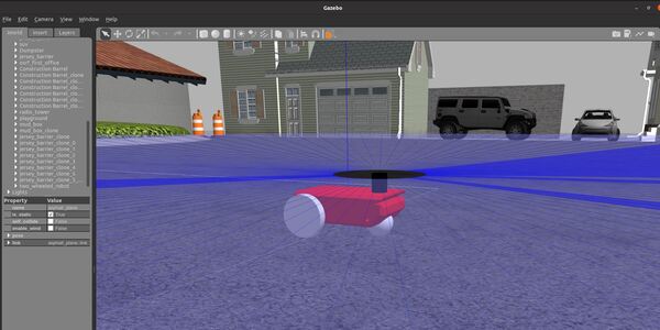
In this tutorial, I will show you how to send a goal path to a mobile robot and the ROS 2 Navigation Stack (also known as Nav2) using Python code. Here is the final output you will be able to achieve after going through this tutorial:
Real-World Applications
The application we will develop in this tutorial has a number of real-world use cases.
For example, you can build an autonomous agricultural robot that can do the following jobs:
- Precision Weeding
- Counting
- Fruit Picking
- Harvesting
- Irrigation
- Monitoring
- Mowing
- Planting
- Pruning
- Seeding
- Spraying
You could also use this application for an autonomous robotic lawn mower.
Prerequisites
- ROS 2 Foxy Fitzroy installed on Ubuntu Linux 20.04 or newer. I am using ROS 2 Galactic, which is the latest version of ROS 2 as of the date of this post.
- You have already created a ROS 2 workspace. The name of our workspace is “dev_ws”, which stands for “development workspace.”
- You have Python 3.7 or higher.
- (Optional) You have completed my Ultimate Guide to the ROS 2 Navigation Stack.
- (Optional) You have a package named two_wheeled_robot inside your ~/dev_ws/src folder, which I set up in this post. If you have another package, that is fine.
- (Optional) You know how to load a world file into Gazebo using ROS 2.
You can find the files for this post here on my Google Drive. Credit to this GitHub repository for the Python scripts. You can find an explanation of Nav2 here.
Directions
Open a terminal window, and move to your package.
cd ~/dev_ws/src/two_wheeled_robot/scripts
Open a new Python program called nav_through_poses.py.
gedit nav_through_poses.py
Add this code.
#! /usr/bin/env python3
# Copyright 2021 Samsung Research America
#
# Licensed under the Apache License, Version 2.0 (the "License");
# you may not use this file except in compliance with the License.
# You may obtain a copy of the License at
#
#     http://www.apache.org/licenses/LICENSE-2.0
#
# Unless required by applicable law or agreed to in writing, software
# distributed under the License is distributed on an "AS IS" BASIS,
# WITHOUT WARRANTIES OR CONDITIONS OF ANY KIND, either express or implied.
# See the License for the specific language governing permissions and
# limitations under the License.
#
# Modified by AutomaticAddison.com

import time # Time library

from geometry_msgs.msg import PoseStamped # Pose with ref frame and timestamp
from rclpy.duration import Duration # Handles time for ROS 2
import rclpy # Python client library for ROS 2

from robot_navigator import BasicNavigator, TaskResult # Helper module

'''
Navigates a robot through goal poses.
'''
def main():

  # Start the ROS 2 Python Client Library
  rclpy.init()


  # Launch the ROS 2 Navigation Stack
  navigator = BasicNavigator()

  # Set the robot's initial pose if necessary
  # initial_pose = PoseStamped()
  # initial_pose.header.frame_id = 'map'
  # initial_pose.header.stamp = navigator.get_clock().now().to_msg()
  # initial_pose.pose.position.x = -6.5
  # initial_pose.pose.position.y = -4.2
  # initial_pose.pose.position.z = 0.0
  # initial_pose.pose.orientation.x = 0.0
  # initial_pose.pose.orientation.y = 0.0
  # initial_pose.pose.orientation.z = 0.0
  # initial_pose.pose.orientation.w = 1.0
  # navigator.setInitialPose(initial_pose)

  # Activate navigation, if not autostarted. This should be called after setInitialPose()
  # or this will initialize at the origin of the map and update the costmap with bogus readings.
  # If autostart, you should `waitUntilNav2Active()` instead.
  # navigator.lifecycleStartup()

  # Wait for navigation to fully activate. Use this line if autostart is set to true.
  navigator.waitUntilNav2Active()

  # If desired, you can change or load the map as well
  # navigator.changeMap('/path/to/map.yaml')

  # You may use the navigator to clear or obtain costmaps
  # navigator.clearAllCostmaps()  # also have clearLocalCostmap() and clearGlobalCostmap()
  # global_costmap = navigator.getGlobalCostmap()
  # local_costmap = navigator.getLocalCostmap()

  # Set the robot's goal poses
  goal_poses = []

  goal_pose = PoseStamped()
  goal_pose.header.frame_id = 'map'
  goal_pose.header.stamp = navigator.get_clock().now().to_msg()
  goal_pose.pose.position.x = -5.0
  goal_pose.pose.position.y = -4.2
  goal_pose.pose.position.z = 0.0
  goal_pose.pose.orientation.x = 0.0
  goal_pose.pose.orientation.y = 0.0
  goal_pose.pose.orientation.z = 0.0
  goal_pose.pose.orientation.w = 1.0
  goal_poses.append(goal_pose)

  goal_pose = PoseStamped()
  goal_pose.header.frame_id = 'map'
  goal_pose.header.stamp = navigator.get_clock().now().to_msg()
  goal_pose.pose.position.x = 0.0
  goal_pose.pose.position.y = -4.2
  goal_pose.pose.position.z = 0.0
  goal_pose.pose.orientation.x = 0.0
  goal_pose.pose.orientation.y = 0.0
  goal_pose.pose.orientation.z = 0.0
  goal_pose.pose.orientation.w = 1.0
  goal_poses.append(goal_pose)

  goal_pose = PoseStamped()
  goal_pose.header.frame_id = 'map'
  goal_pose.header.stamp = navigator.get_clock().now().to_msg()
  goal_pose.pose.position.x = 5.0
  goal_pose.pose.position.y = -4.2
  goal_pose.pose.position.z = 0.0
  goal_pose.pose.orientation.x = 0.0
  goal_pose.pose.orientation.y = 0.0
  goal_pose.pose.orientation.z = 0.0
  goal_pose.pose.orientation.w = 1.0
  goal_poses.append(goal_pose)

  goal_pose = PoseStamped()
  goal_pose.header.frame_id = 'map'
  goal_pose.header.stamp = navigator.get_clock().now().to_msg()
  goal_pose.pose.position.x = 10.0
  goal_pose.pose.position.y = -4.2
  goal_pose.pose.position.z = 0.0
  goal_pose.pose.orientation.x = 0.0
  goal_pose.pose.orientation.y = 0.0
  goal_pose.pose.orientation.z = 0.0
  goal_pose.pose.orientation.w = 1.0
  goal_poses.append(goal_pose)

  goal_pose = PoseStamped()
  goal_pose.header.frame_id = 'map'
  goal_pose.header.stamp = navigator.get_clock().now().to_msg()
  goal_pose.pose.position.x = 13.0
  goal_pose.pose.position.y = -4.2
  goal_pose.pose.position.z = 0.0
  goal_pose.pose.orientation.x = 0.0
  goal_pose.pose.orientation.y = 0.0
  goal_pose.pose.orientation.z = 0.0
  goal_pose.pose.orientation.w = 1.0
  goal_poses.append(goal_pose)

  goal_pose = PoseStamped()
  goal_pose.header.frame_id = 'map'
  goal_pose.header.stamp = navigator.get_clock().now().to_msg()
  goal_pose.pose.position.x = 13.5
  goal_pose.pose.position.y = -3.7
  goal_pose.pose.position.z = 0.0
  goal_pose.pose.orientation.x = 0.0
  goal_pose.pose.orientation.y = 0.0
  goal_pose.pose.orientation.z = 0.38
  goal_pose.pose.orientation.w = 0.92
  goal_poses.append(goal_pose)

  goal_pose = PoseStamped()
  goal_pose.header.frame_id = 'map'
  goal_pose.header.stamp = navigator.get_clock().now().to_msg()
  goal_pose.pose.position.x = 13.5
  goal_pose.pose.position.y = -3.2
  goal_pose.pose.position.z = 0.0
  goal_pose.pose.orientation.x = 0.0
  goal_pose.pose.orientation.y = 0.0
  goal_pose.pose.orientation.z = 0.707
  goal_pose.pose.orientation.w = 0.707
  goal_poses.append(goal_pose)

  goal_pose = PoseStamped()
  goal_pose.header.frame_id = 'map'
  goal_pose.header.stamp = navigator.get_clock().now().to_msg()
  goal_pose.pose.position.x = 13.5
  goal_pose.pose.position.y = -2.7
  goal_pose.pose.position.z = 0.0
  goal_pose.pose.orientation.x = 0.0
  goal_pose.pose.orientation.y = 0.0
  goal_pose.pose.orientation.z = 0.92
  goal_pose.pose.orientation.w = 0.38
  goal_poses.append(goal_pose)

  goal_pose = PoseStamped()
  goal_pose.header.frame_id = 'map'
  goal_pose.header.stamp = navigator.get_clock().now().to_msg()
  goal_pose.pose.position.x = 13.0
  goal_pose.pose.position.y = -2.2
  goal_pose.pose.position.z = 0.0
  goal_pose.pose.orientation.x = 0.0
  goal_pose.pose.orientation.y = 0.0
  goal_pose.pose.orientation.z = 1.0
  goal_pose.pose.orientation.w = 0.0
  goal_poses.append(goal_pose)

  goal_pose = PoseStamped()
  goal_pose.header.frame_id = 'map'
  goal_pose.header.stamp = navigator.get_clock().now().to_msg()
  goal_pose.pose.position.x = 10.0
  goal_pose.pose.position.y = -2.2
  goal_pose.pose.position.z = 0.0
  goal_pose.pose.orientation.x = 0.0
  goal_pose.pose.orientation.y = 0.0
  goal_pose.pose.orientation.z = 1.0
  goal_pose.pose.orientation.w = 0.0
  goal_poses.append(goal_pose)

  goal_pose = PoseStamped()
  goal_pose.header.frame_id = 'map'
  goal_pose.header.stamp = navigator.get_clock().now().to_msg()
  goal_pose.pose.position.x = 5.0
  goal_pose.pose.position.y = -2.2
  goal_pose.pose.position.z = 0.0
  goal_pose.pose.orientation.x = 0.0
  goal_pose.pose.orientation.y = 0.0
  goal_pose.pose.orientation.z = 1.0
  goal_pose.pose.orientation.w = 0.0
  goal_poses.append(goal_pose)

  goal_pose = PoseStamped()
  goal_pose.header.frame_id = 'map'
  goal_pose.header.stamp = navigator.get_clock().now().to_msg()
  goal_pose.pose.position.x = 0.0
  goal_pose.pose.position.y = -2.2
  goal_pose.pose.position.z = 0.0
  goal_pose.pose.orientation.x = 0.0
  goal_pose.pose.orientation.y = 0.0
  goal_pose.pose.orientation.z = 1.0
  goal_pose.pose.orientation.w = 0.0
  goal_poses.append(goal_pose)

  goal_pose = PoseStamped()
  goal_pose.header.frame_id = 'map'
  goal_pose.header.stamp = navigator.get_clock().now().to_msg()
  goal_pose.pose.position.x = -5.0
  goal_pose.pose.position.y = -2.2
  goal_pose.pose.position.z = 0.0
  goal_pose.pose.orientation.x = 0.0
  goal_pose.pose.orientation.y = 0.0
  goal_pose.pose.orientation.z = 1.0
  goal_pose.pose.orientation.w = 0.0
  goal_poses.append(goal_pose)

  goal_pose = PoseStamped()
  goal_pose.header.frame_id = 'map'
  goal_pose.header.stamp = navigator.get_clock().now().to_msg()
  goal_pose.pose.position.x = -6.5
  goal_pose.pose.position.y = -2.2
  goal_pose.pose.position.z = 0.0
  goal_pose.pose.orientation.x = 0.0
  goal_pose.pose.orientation.y = 0.0
  goal_pose.pose.orientation.z = 1.0
  goal_pose.pose.orientation.w = 0.0
  goal_poses.append(goal_pose)

  goal_pose = PoseStamped()
  goal_pose.header.frame_id = 'map'
  goal_pose.header.stamp = navigator.get_clock().now().to_msg()
  goal_pose.pose.position.x = -7.0
  goal_pose.pose.position.y = -1.7
  goal_pose.pose.position.z = 0.0
  goal_pose.pose.orientation.x = 0.0
  goal_pose.pose.orientation.y = 0.0
  goal_pose.pose.orientation.z = 0.92
  goal_pose.pose.orientation.w = 0.38
  goal_poses.append(goal_pose)

  goal_pose = PoseStamped()
  goal_pose.header.frame_id = 'map'
  goal_pose.header.stamp = navigator.get_clock().now().to_msg()
  goal_pose.pose.position.x = -7.0
  goal_pose.pose.position.y = -1.2
  goal_pose.pose.position.z = 0.0
  goal_pose.pose.orientation.x = 0.0
  goal_pose.pose.orientation.y = 0.0
  goal_pose.pose.orientation.z = 0.707
  goal_pose.pose.orientation.w = 0.707
  goal_poses.append(goal_pose)

  goal_pose = PoseStamped()
  goal_pose.header.frame_id = 'map'
  goal_pose.header.stamp = navigator.get_clock().now().to_msg()
  goal_pose.pose.position.x = -7.0
  goal_pose.pose.position.y = -0.7
  goal_pose.pose.position.z = 0.0
  goal_pose.pose.orientation.x = 0.0
  goal_pose.pose.orientation.y = 0.0
  goal_pose.pose.orientation.z = 0.38
  goal_pose.pose.orientation.w = 0.92
  goal_poses.append(goal_pose)

  goal_pose = PoseStamped()
  goal_pose.header.frame_id = 'map'
  goal_pose.header.stamp = navigator.get_clock().now().to_msg()
  goal_pose.pose.position.x = -6.5
  goal_pose.pose.position.y = 0.0
  goal_pose.pose.position.z = 0.0
  goal_pose.pose.orientation.x = 0.0
  goal_pose.pose.orientation.y = 0.0
  goal_pose.pose.orientation.z = 0.0
  goal_pose.pose.orientation.w = 1.0
  goal_poses.append(goal_pose)

  goal_pose = PoseStamped()
  goal_pose.header.frame_id = 'map'
  goal_pose.header.stamp = navigator.get_clock().now().to_msg()
  goal_pose.pose.position.x = -5.0
  goal_pose.pose.position.y = 0.0
  goal_pose.pose.position.z = 0.0
  goal_pose.pose.orientation.x = 0.0
  goal_pose.pose.orientation.y = 0.0
  goal_pose.pose.orientation.z = 0.0
  goal_pose.pose.orientation.w = 1.0
  goal_poses.append(goal_pose)

  goal_pose = PoseStamped()
  goal_pose.header.frame_id = 'map'
  goal_pose.header.stamp = navigator.get_clock().now().to_msg()
  goal_pose.pose.position.x = 0.0
  goal_pose.pose.position.y = 0.0
  goal_pose.pose.position.z = 0.0
  goal_pose.pose.orientation.x = 0.0
  goal_pose.pose.orientation.y = 0.0
  goal_pose.pose.orientation.z = 0.0
  goal_pose.pose.orientation.w = 1.0
  goal_poses.append(goal_pose)

  goal_pose = PoseStamped()
  goal_pose.header.frame_id = 'map'
  goal_pose.header.stamp = navigator.get_clock().now().to_msg()
  goal_pose.pose.position.x = 5.0
  goal_pose.pose.position.y = 0.0
  goal_pose.pose.position.z = 0.0
  goal_pose.pose.orientation.x = 0.0
  goal_pose.pose.orientation.y = 0.0
  goal_pose.pose.orientation.z = 0.0
  goal_pose.pose.orientation.w = 1.0
  goal_poses.append(goal_pose)

  goal_pose = PoseStamped()
  goal_pose.header.frame_id = 'map'
  goal_pose.header.stamp = navigator.get_clock().now().to_msg()
  goal_pose.pose.position.x = 10.0
  goal_pose.pose.position.y = 0.0
  goal_pose.pose.position.z = 0.0
  goal_pose.pose.orientation.x = 0.0
  goal_pose.pose.orientation.y = 0.0
  goal_pose.pose.orientation.z = 0.0
  goal_pose.pose.orientation.w = 1.0
  goal_poses.append(goal_pose)

  goal_pose5 = PoseStamped()
  goal_pose5.header.frame_id = 'map'
  goal_pose5.header.stamp = navigator.get_clock().now().to_msg()
  goal_pose5.pose.position.x = 13.0
  goal_pose5.pose.position.y = 0.0
  goal_pose5.pose.position.z = 0.0
  goal_pose5.pose.orientation.x = 0.0
  goal_pose5.pose.orientation.y = 0.0
  goal_pose5.pose.orientation.z = 0.0
  goal_pose5.pose.orientation.w = 1.0
  goal_poses.append(goal_pose5)

  goal_pose = PoseStamped()
  goal_pose.header.frame_id = 'map'
  goal_pose.header.stamp = navigator.get_clock().now().to_msg()
  goal_pose.pose.position.x = 13.5
  goal_pose.pose.position.y = 0.5
  goal_pose.pose.position.z = 0.0
  goal_pose.pose.orientation.x = 0.0
  goal_pose.pose.orientation.y = 0.0
  goal_pose.pose.orientation.z = 0.38
  goal_pose.pose.orientation.w = 0.92
  goal_poses.append(goal_pose)

  goal_pose = PoseStamped()
  goal_pose.header.frame_id = 'map'
  goal_pose.header.stamp = navigator.get_clock().now().to_msg()
  goal_pose.pose.position.x = 13.5
  goal_pose.pose.position.y = 1.0
  goal_pose.pose.position.z = 0.0
  goal_pose.pose.orientation.x = 0.0
  goal_pose.pose.orientation.y = 0.0
  goal_pose.pose.orientation.z = 0.707
  goal_pose.pose.orientation.w = 0.707
  goal_poses.append(goal_pose)

  goal_pose = PoseStamped()
  goal_pose.header.frame_id = 'map'
  goal_pose.header.stamp = navigator.get_clock().now().to_msg()
  goal_pose.pose.position.x = 13.5
  goal_pose.pose.position.y = 1.5
  goal_pose.pose.position.z = 0.0
  goal_pose.pose.orientation.x = 0.0
  goal_pose.pose.orientation.y = 0.0
  goal_pose.pose.orientation.z = 0.92
  goal_pose.pose.orientation.w = 0.38
  goal_poses.append(goal_pose)

  goal_pose = PoseStamped()
  goal_pose.header.frame_id = 'map'
  goal_pose.header.stamp = navigator.get_clock().now().to_msg()
  goal_pose.pose.position.x = 13.0
  goal_pose.pose.position.y = 2.2
  goal_pose.pose.position.z = 0.0
  goal_pose.pose.orientation.x = 0.0
  goal_pose.pose.orientation.y = 0.0
  goal_pose.pose.orientation.z = 1.0
  goal_pose.pose.orientation.w = 0.0
  goal_poses.append(goal_pose)

  goal_pose = PoseStamped()
  goal_pose.header.frame_id = 'map'
  goal_pose.header.stamp = navigator.get_clock().now().to_msg()
  goal_pose.pose.position.x = 10.0
  goal_pose.pose.position.y = 2.2
  goal_pose.pose.position.z = 0.0
  goal_pose.pose.orientation.x = 0.0
  goal_pose.pose.orientation.y = 0.0
  goal_pose.pose.orientation.z = 1.0
  goal_pose.pose.orientation.w = 0.0
  goal_poses.append(goal_pose)

  goal_pose = PoseStamped()
  goal_pose.header.frame_id = 'map'
  goal_pose.header.stamp = navigator.get_clock().now().to_msg()
  goal_pose.pose.position.x = 5.0
  goal_pose.pose.position.y = 2.2
  goal_pose.pose.position.z = 0.0
  goal_pose.pose.orientation.x = 0.0
  goal_pose.pose.orientation.y = 0.0
  goal_pose.pose.orientation.z = 1.0
  goal_pose.pose.orientation.w = 0.0
  goal_poses.append(goal_pose)

  goal_pose = PoseStamped()
  goal_pose.header.frame_id = 'map'
  goal_pose.header.stamp = navigator.get_clock().now().to_msg()
  goal_pose.pose.position.x = 0.0
  goal_pose.pose.position.y = 2.2
  goal_pose.pose.position.z = 0.0
  goal_pose.pose.orientation.x = 0.0
  goal_pose.pose.orientation.y = 0.0
  goal_pose.pose.orientation.z = 1.0
  goal_pose.pose.orientation.w = 0.0
  goal_poses.append(goal_pose)

  goal_pose = PoseStamped()
  goal_pose.header.frame_id = 'map'
  goal_pose.header.stamp = navigator.get_clock().now().to_msg()
  goal_pose.pose.position.x = -5.0
  goal_pose.pose.position.y = 2.2
  goal_pose.pose.position.z = 0.0
  goal_pose.pose.orientation.x = 0.0
  goal_pose.pose.orientation.y = 0.0
  goal_pose.pose.orientation.z = 1.0
  goal_pose.pose.orientation.w = 0.0
  goal_poses.append(goal_pose)

  goal_pose = PoseStamped()
  goal_pose.header.frame_id = 'map'
  goal_pose.header.stamp = navigator.get_clock().now().to_msg()
  goal_pose.pose.position.x = -6.5
  goal_pose.pose.position.y = 2.2
  goal_pose.pose.position.z = 0.0
  goal_pose.pose.orientation.x = 0.0
  goal_pose.pose.orientation.y = 0.0
  goal_pose.pose.orientation.z = 1.0
  goal_pose.pose.orientation.w = 0.0
  goal_poses.append(goal_pose)

  goal_pose = PoseStamped()
  goal_pose.header.frame_id = 'map'
  goal_pose.header.stamp = navigator.get_clock().now().to_msg()
  goal_pose.pose.position.x = -7.0
  goal_pose.pose.position.y = 2.7
  goal_pose.pose.position.z = 0.0
  goal_pose.pose.orientation.x = 0.0
  goal_pose.pose.orientation.y = 0.0
  goal_pose.pose.orientation.z = 0.92
  goal_pose.pose.orientation.w = 0.38
  goal_poses.append(goal_pose)

  goal_pose = PoseStamped()
  goal_pose.header.frame_id = 'map'
  goal_pose.header.stamp = navigator.get_clock().now().to_msg()
  goal_pose.pose.position.x = -7.0
  goal_pose.pose.position.y = 3.2
  goal_pose.pose.position.z = 0.0
  goal_pose.pose.orientation.x = 0.0
  goal_pose.pose.orientation.y = 0.0
  goal_pose.pose.orientation.z = 0.707
  goal_pose.pose.orientation.w = 0.707
  goal_poses.append(goal_pose)

  goal_pose = PoseStamped()
  goal_pose.header.frame_id = 'map'
  goal_pose.header.stamp = navigator.get_clock().now().to_msg()
  goal_pose.pose.position.x = -7.0
  goal_pose.pose.position.y = 3.7
  goal_pose.pose.position.z = 0.0
  goal_pose.pose.orientation.x = 0.0
  goal_pose.pose.orientation.y = 0.0
  goal_pose.pose.orientation.z = 0.38
  goal_pose.pose.orientation.w = 0.92
  goal_poses.append(goal_pose)

  goal_pose = PoseStamped()
  goal_pose.header.frame_id = 'map'
  goal_pose.header.stamp = navigator.get_clock().now().to_msg()
  goal_pose.pose.position.x = -6.5
  goal_pose.pose.position.y = 4.2
  goal_pose.pose.position.z = 0.0
  goal_pose.pose.orientation.x = 0.0
  goal_pose.pose.orientation.y = 0.0
  goal_pose.pose.orientation.z = 0.0
  goal_pose.pose.orientation.w = 1.0
  goal_poses.append(goal_pose)

  goal_pose = PoseStamped()
  goal_pose.header.frame_id = 'map'
  goal_pose.header.stamp = navigator.get_clock().now().to_msg()
  goal_pose.pose.position.x = -5.0
  goal_pose.pose.position.y = 4.2
  goal_pose.pose.position.z = 0.0
  goal_pose.pose.orientation.x = 0.0
  goal_pose.pose.orientation.y = 0.0
  goal_pose.pose.orientation.z = 0.0
  goal_pose.pose.orientation.w = 1.0
  goal_poses.append(goal_pose)

  goal_pose = PoseStamped()
  goal_pose.header.frame_id = 'map'
  goal_pose.header.stamp = navigator.get_clock().now().to_msg()
  goal_pose.pose.position.x = 0.0
  goal_pose.pose.position.y = 4.2
  goal_pose.pose.position.z = 0.0
  goal_pose.pose.orientation.x = 0.0
  goal_pose.pose.orientation.y = 0.0
  goal_pose.pose.orientation.z = 0.0
  goal_pose.pose.orientation.w = 1.0
  goal_poses.append(goal_pose)

  goal_pose = PoseStamped()
  goal_pose.header.frame_id = 'map'
  goal_pose.header.stamp = navigator.get_clock().now().to_msg()
  goal_pose.pose.position.x = 5.0
  goal_pose.pose.position.y = 4.2
  goal_pose.pose.position.z = 0.0
  goal_pose.pose.orientation.x = 0.0
  goal_pose.pose.orientation.y = 0.0
  goal_pose.pose.orientation.z = 0.0
  goal_pose.pose.orientation.w = 1.0
  goal_poses.append(goal_pose)

  goal_pose = PoseStamped()
  goal_pose.header.frame_id = 'map'
  goal_pose.header.stamp = navigator.get_clock().now().to_msg()
  goal_pose.pose.position.x = 10.0
  goal_pose.pose.position.y = 4.2
  goal_pose.pose.position.z = 0.0
  goal_pose.pose.orientation.x = 0.0
  goal_pose.pose.orientation.y = 0.0
  goal_pose.pose.orientation.z = 0.0
  goal_pose.pose.orientation.w = 1.0
  goal_poses.append(goal_pose)

  goal_pose = PoseStamped()
  goal_pose.header.frame_id = 'map'
  goal_pose.header.stamp = navigator.get_clock().now().to_msg()
  goal_pose.pose.position.x = 13.0
  goal_pose.pose.position.y = 4.2
  goal_pose.pose.position.z = 0.0
  goal_pose.pose.orientation.x = 0.0
  goal_pose.pose.orientation.y = 0.0
  goal_pose.pose.orientation.z = 0.0
  goal_pose.pose.orientation.w = 1.0
  goal_poses.append(goal_pose)

  # sanity check a valid path exists
  # path = navigator.getPathThroughPoses(initial_pose, goal_poses)

  # Go through the goal poses
  navigator.goThroughPoses(goal_poses)

  i = 0
  # Keep doing stuff as long as the robot is moving towards the goal poses
  while not navigator.isNavComplete():
    ################################################
    #
    # Implement some code here for your application!
    #
    ################################################

    # Do something with the feedback
    i = i + 1
    feedback = navigator.getFeedback()
    if feedback and i % 5 == 0:
      print('Distance remaining: ' + '{:.2f}'.format(
            feedback.distance_remaining) + ' meters.')

      # Some navigation timeout to demo cancellation
      if Duration.from_msg(feedback.navigation_time) > Duration(seconds=1000000.0):
        navigator.cancelNav()

      # Some navigation request change to demo preemption
      if Duration.from_msg(feedback.navigation_time) > Duration(seconds=500000.0):
        goal_pose_alt = PoseStamped()
        goal_pose_alt.header.frame_id = 'map'
        goal_pose_alt.header.stamp = navigator.get_clock().now().to_msg()
        goal_pose_alt.pose.position.x = -6.5
        goal_pose_alt.pose.position.y = -4.2
        goal_pose_alt.pose.position.z = 0.0
        goal_pose_alt.pose.orientation.x = 0.0
        goal_pose_alt.pose.orientation.y = 0.0
        goal_pose_alt.pose.orientation.z = 0.0
        goal_pose_alt.pose.orientation.w = 1.0
        navigator.goThroughPoses([goal_pose_alt])

  # Do something depending on the return code
  result = navigator.getResult()
  if result == TaskResult.SUCCEEDED:
    print('Goal succeeded!')
  elif result == TaskResult.CANCELED:
    print('Goal was canceled!')
  elif result == TaskResult.FAILED:
    print('Goal failed!')
  else:
    print('Goal has an invalid return status!')

  # Close the ROS 2 Navigation Stack
  navigator.lifecycleShutdown()

  exit(0)

if __name__ == '__main__':
  main()
The orientation values are in quaternion format. You can use this calculator to convert from Euler angles (e.g. x = 0 radians, y = 0 radians, z = 1.57 radians) to quaternion format (e.g. x = 0, y, = 0, z = 0.707, w = 0.707).
Save the code, and close the file.
Change the access permissions on the file.
chmod +x nav_through_poses.py
Open a new Python program called robot_navigator.py.
gedit robot_navigator.py
Add this code.
Save the code and close the file.
Change the access permissions on the file.
chmod +x robot_navigator.py
Open CMakeLists.txt.
cd ~/dev_ws/src/two_wheeled_robot
gedit CMakeLists.txt
Add the Python executables. Here is what my CMakeLists.txt file looks like.
scripts/nav_through_poses.py
scripts/robot_navigator.py
Add the launch file. Here is my launch file code.
cd ~/dev_ws/src/two_wheeled_robot/launch/farm_world
gedit farm_world_v2.launch.py
Save and close the file.
Add the Nav2 parameters.
cd ~/dev_ws/src/two_wheeled_robot/params/farm_world
gedit nav2_params_static_transform_pub.yaml
Save and close the file.
Now we build the package.
cd ~/dev_ws/
colcon build
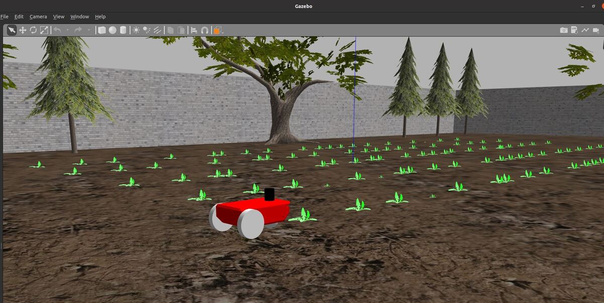
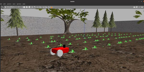
Open a new terminal and launch the robot in a Gazebo world. I chose to use my farm_world that has several rows of crops.
ros2 launch two_wheeled_robot farm_world_v2.launch.py
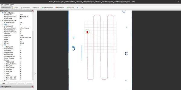
Wait for the simulation to fully load. I like to wait three minutes so the pose of the robot can set to the correct location within RViz.
If the global costmap doesn’t load, try launching again.
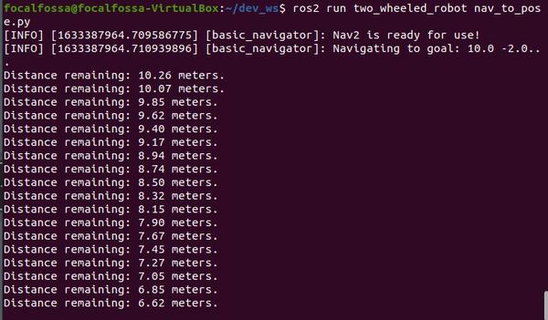
Now send the goal path by opening a new terminal window, and typing:
ros2 run two_wheeled_robot nav_through_poses.py
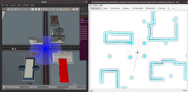
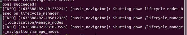
You will see the distance remaining to the goal pose printed on the screen. You can also choose to print other information to the screen by getting the appropriate message type.
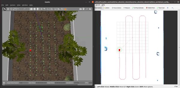
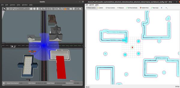
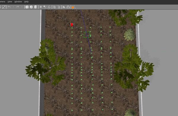
You will also see the path from the initial pose to the goal poses printed on the screen.
The robot will move through the goal poses.
A success message will print once the robot has reached the final goal pose.
That’s it! Keep building!