

In this tutorial, we will go over how to create a Python publisher for ROS 2.
In ROS 2 (Robot Operating System 2), a Python publisher is a program or script (written in Python) that sends messages across the ROS network to other parts of the system.
The official instructions for creating a publisher are here, but I will walk you through the entire process, step by step.
We will be following the ROS 2 Python Style Guide.
Let’s get started!
Prerequisites
- You have created a ROS 2 workspace.
- You have created a ROS 2 package.
- You have Visual Studio code installed.
- Code is stored here on GitHub.
Directions
Open a terminal, and type these commands to open VS Code.
cd ~/ros2_wscode .You can close any pop ups that appear.
Let’s set our default indentation to 4 spaces.
Here are the steps to set a default 4-space indentation in VS Code:
1. Access Settings:
- Using the menu: Go to File > Preferences > Settings (or press Ctrl+, on Windows/Linux or Cmd+, on macOS).
2. Modify Settings:
- Search for “Indentation” in the settings panel.
- Change the following values:
- “Editor: Tab Size”: Set this to 4 to control the width of a tab character.
- “Editor: Insert Spaces”: Set this to true to ensure that pressing Tab inserts spaces instead of a literal tab character.
- (Optional) “Editor: Detect Indentation”: Set this to false if you want to prevent VS Code from automatically adjusting indentation based on existing code.
3. Apply Changes:
- The changes should take effect immediately. You can test by opening a file and pressing Tab to see if it inserts 4 spaces.
Write the Code
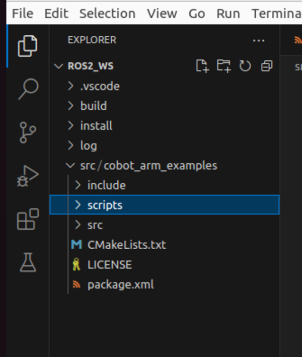
Right-click on src/cobot_arm_examples, and type “scripts” to create a new folder for our Python script.
Right-click on the scripts folder to create a new file called “minimal_py_publisher.py”.
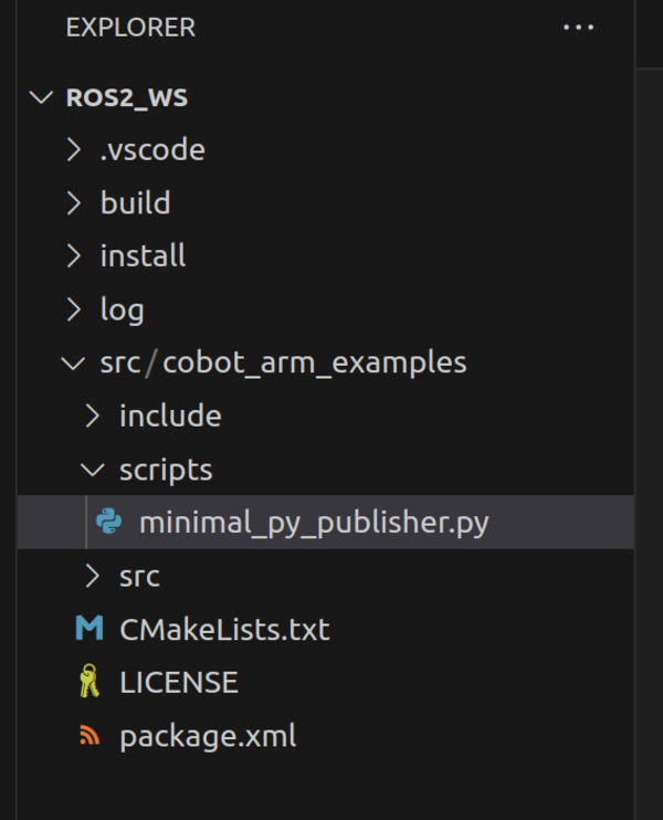
Type the following code inside minimal_py_publisher.py:
#! /usr/bin/env python3

"""
Description:
    This ROS 2 node periodically publishes "Hello World" messages on a topic.
    It demonstrates basic ROS concepts such as node creation, publishing, and
    timer usage.
-------
Publishing Topics:
    The channel containing the "Hello World" messages
    /topic - std_msgs/String
-------
Subscription Topics:
    None
-------
Author: Addison Sears-Collins
Date: January 31, 2024
"""

import rclpy # Import the ROS 2 client library for Python
from rclpy.node import Node # Import the Node class for creating ROS 2 nodes

from std_msgs.msg import String # Import the String message type for publishing


class MinimalPublisher(Node):
    """Create MinimalPublisher node.

    """
    def __init__(self):
        """ Create a custom node class for publishing messages

        """

        # Initialize the node with a name
        super().__init__('minimal_publisher')

        # Creates a publisher on the topic "topic" with a queue size of 10 messages
        self.publisher_1 = self.create_publisher(String, '/topic', 10)

        # Create a timer with a period of 0.5 seconds to trigger the callback function
        timer_period = 0.5  # seconds
        self.timer = self.create_timer(timer_period, self.timer_callback)

        # Initialize a counter variable for message content
        self.i = 0

    def timer_callback(self):
        """Callback function executed periodically by the timer.

        """
        # Create a new String message object
        msg = String()

        # Set the message data with a counter
        msg.data = 'Hello World: %d' % self.i

        # Publish the message on the topic
        self.publisher_1.publish(msg)

        # Log a message indicating that the message has been published
        self.get_logger().info('Publishing: "%s"' % msg.data)

        # Increment the counter for the next message
        self.i = self.i + 1


def main(args=None):
    """Main function to start the ROS 2 node.

    Args:
        args (List, optional): Command-line arguments. Defaults to None.
    """

    # Initialize ROS 2 communication
    rclpy.init(args=args)

    # Create an instance of the MinimalPublisher node
    minimal_publisher = MinimalPublisher()

    # Keep the node running and processing events.
    rclpy.spin(minimal_publisher)

    # Destroy the node explicitly
    # (optional - otherwise it will be done automatically
    # when the garbage collector destroys the node object)
    minimal_publisher.destroy_node()

    # Shutdown ROS 2 communication
    rclpy.shutdown()

if __name__ == '__main__':
    # Execute the main function if the script is run directly
    main()
To generate the comments for each class and function, you follow these steps for the autoDocstring package.
What we are going to do in this node is publish the string “Hello World” to a topic named /topic. The string message will also contain a counter that keeps track of how many times the message has been published.
We chose the name /topic for the topic, but you could have chosen any name.
Configure the Package
Create the __init__.py file
Now, we need to configure our package so that ROS 2 can discover this Python node we just created.
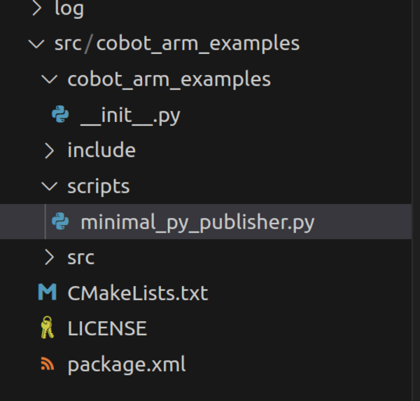
Right-click on src/cobot_arm_examples, and create a folder that has the same name as the package. This folder is required in order to run Python scripts.
ROS 2’s build system, ament, relies on this structure to correctly locate and build Python modules within a package. The folder with the same name as the package serves as the root for Python code, allowing ament to accurately generate and install the package’s Python modules.
Now right-click on the name of this folder, and create an empty script called
__init__.py.Here is what the file should look like:
# Required to import Python modules
The presence of _ _init_ _.py explicitly designates a directory as a Python package. This enables Python’s import machinery to recognize and treat it as a cohesive collection of modules.
Create a README.md
Now let’s create a README.md file. Right-click on the name of the package, and name the file README.md.
A README.md file is a plain text file that serves as an introduction and explanation for a project, software, or package. It’s like a welcome mat for anyone encountering your work, providing essential information and guidance to get them started.
You can find a syntax guide on how to write a README.md file here on GitHub.
# cobot_arm_examples

This package provides some basic examples to get you started with ROS 2 manipulation.
To see what the README.md file looks like, you can right-click on README.md on the left pane and click “Open Preview”.
Modify the package.xml File
Now let’s open the package.xml file. Make sure it looks like this.
<?xml version="1.0"?>
<?xml-model href="http://download.ros.org/schema/package_format3.xsd" schematypens="http://www.w3.org/2001/XMLSchema"?>
<package format="3">
  <name>cobot_arm_examples</name>
  <version>0.0.0</version>
  <description>Basic examples demonstrating ROS 2</description>
  <maintainer email="automaticaddison@example.com">Addison Sears-Collins</maintainer>
  <license>Apache-2.0</license>

  <!--Specify build tools that are needed to compile the package-->
  <buildtool_depend>ament_cmake</buildtool_depend>
  <buildtool_depend>ament_cmake_python</buildtool_depend>

  <!--Declares package dependencies that are required for building the package-->
  <depend>rclcpp</depend>
  <depend>rclpy</depend>
  <depend>std_msgs</depend>

  <!--Specifies dependencies that are only needed for testing the package-->
  <test_depend>ament_lint_auto</test_depend>
  <test_depend>ament_lint_common</test_depend>

  <export>
    <build_type>ament_cmake</build_type>
  </export>
</package>
The package.xml file is an important part of any ROS 2 package. It serves as the package’s manifest, holding essential metadata that ROS 2 tools use to build, install, and manage the package.
Here’s a breakdown of the key elements you’ll find in a typical package.xml file:
1. Basic Information:
- name: The unique identifier for the package, often corresponding to the folder name.
- version: The package’s semantic version, indicating its maturity and compatibility.
- description: A brief explanation of the package’s purpose and functionality.
2. Dependencies:
- build_depend: Packages and libraries required for building the current package.
- buildtool_depend: Build tools (like compilers) needed for building the package.
- run_depend: Packages and libraries required for running the package’s executables.
3. Build Configuration:
- build_type: Specifies the build system (e.g., cmake, catkin).
- export: Defines properties and settings used during package installation.
4. Maintainers and License:
- maintainer: Information about the package’s primary developers and maintainers.
- license: The license under which the package is released (e.g., Apache 2.0).
Modify the CMakeLists.txt File
Now let’s configure the CMakeLists.txt file. A CMakeLists.txt file in ROS 2 defines how a ROS 2 package should be built. It contains instructions for building and linking the package’s executables, libraries, and other artifacts.
cmake_minimum_required(VERSION 3.8)
project(cobot_arm_examples)

# Check if the compiler being used is GNU's C++ compiler (g++) or Clang.
# Add compiler flags for all targets that will be defined later in the
# CMakeLists file. These flags enable extra warnings to help catch
# potential issues in the code.
# Add options to the compilation process
if(CMAKE_COMPILER_IS_GNUCXX OR CMAKE_CXX_COMPILER_ID MATCHES "Clang")
  add_compile_options(-Wall -Wextra -Wpedantic)
endif()

# Locate and configure packages required by the project.
find_package(ament_cmake REQUIRED)
find_package(ament_cmake_python REQUIRED)
find_package(rclcpp REQUIRED)
find_package(rclpy REQUIRED)
find_package(std_msgs REQUIRED)

# Define a CMake variable named dependencies that lists all
# ROS 2 packages and other dependencies the project requires.
set(dependencies
  rclcpp
  std_msgs
)

# Add the specified directories to the list of paths that the compiler
# uses to search for header files. This is important for C++
# projects where you have custom header files that are not located
# in the standard system include paths.
include_directories(
  include
)

# Tells CMake to create an executable target named minimal_cpp_publisher
# from the source file src/minimal_cpp_publisher.cpp. Also make sure CMake
# knows about the program's dependencies.
add_executable(minimal_cpp_publisher src/minimal_cpp_publisher.cpp)
ament_target_dependencies(minimal_cpp_publisher ${dependencies})

add_executable(minimal_cpp_subscriber src/minimal_cpp_subscriber.cpp)
ament_target_dependencies(minimal_cpp_subscriber ${dependencies})

# Copy necessary files to designated locations in the project
install (
  DIRECTORY cobot_arm_examples scripts
  DESTINATION share/${PROJECT_NAME}
)

install(
  DIRECTORY include/
  DESTINATION include
)

# Install cpp executables
install(
  TARGETS
  minimal_cpp_publisher
  minimal_cpp_subscriber
  DESTINATION lib/${PROJECT_NAME}
)

# Install Python modules for import
ament_python_install_package(${PROJECT_NAME})

# Install Python executables
install(
  PROGRAMS
  scripts/minimal_py_publisher.py
  scripts/minimal_py_subscriber.py
  #scripts/example3.py
  #scripts/example4.py
  #scripts/example5.py
  #scripts/example6.py
  #scripts/example7.py
  DESTINATION lib/${PROJECT_NAME}
)

# Automates the process of setting up linting for the package, which
# is the process of running tools that analyze the code for potential
# errors, style issues, and other discrepancies that do not adhere to
# specified coding standards or best practices.
if(BUILD_TESTING)
  find_package(ament_lint_auto REQUIRED)
  # the following line skips the linter which checks for copyrights
  # comment the line when a copyright and license is added to all source files
  set(ament_cmake_copyright_FOUND TRUE)
  # the following line skips cpplint (only works in a git repo)
  # comment the line when this package is in a git repo and when
  # a copyright and license is added to all source files
  set(ament_cmake_cpplint_FOUND TRUE)
  ament_lint_auto_find_test_dependencies()
endif()

# Used to export include directories of a package so that they can be easily
# included by other packages that depend on this package.
ament_export_include_directories(include)

# Generate and install all the necessary CMake and environment hooks that
# allow other packages to find and use this package.
ament_package()
The standard sections of a CMakeLists.txt file for ROS 2 are as follows:
1. cmake_minimum_required:
cmake_minimum_required(VERSION 3.5)
Specifies the minimum required version of CMake for building the package. This is typically set to a version that is known to be compatible with ROS 2.
2. project:
project(my_package)
Specifies the name of the project (ROS 2 package). This sets up various project-related variables and settings.
3. find_package:
find_package(ament_cmake REQUIRED)
Finds and loads the necessary dependencies for the ROS 2 package. `ament_cmake` is a key package used in ROS 2 build systems.
4. ament_package:
ament_package()
Configures the package to use the appropriate ROS 2 build and install infrastructure. This line should be present at the end of the `CMakeLists.txt` file.
5. add_executable or add_library:
add_executable(my_node src/my_node.cpp)
Defines an executable or a library to be built. This command specifies the source files associated with the target.
6. ament_target_dependencies:
ament_target_dependencies(my_node rclcpp)
Declares the dependencies for a target (executable or library). In this example, `my_node` depends on the `rclcpp` library.
7. install:
install(TARGETS
my_node
DESTINATION lib/${PROJECT_NAME})
Specifies the installation rules for the built artifacts. It defines where the executable or library should be installed.
8. ament_export_dependencies:
ament_export_dependencies(ament_cmake)
Exports the dependencies of the package. This is used to inform downstream packages about the dependencies of the current package.
9. ament_export_include_directories:
ament_export_include_directories(include)
Exports the include directories of the package. This is used to inform downstream packages about the include directories.
10. ament_export_libraries:
ament_export_libraries(my_library)
Exports the libraries of the package. This is used to inform downstream packages about the libraries.
11. ament_package_config_dependency:
ament_package_config_dependency(rclcpp)
Declares a dependency on another package for the purpose of package configuration. This is used when configuring the package for building against other packages.
These sections collectively define the build process, dependencies, and installation rules for a ROS 2 package. The specific content within each section will vary depending on the package’s requirements and structure.
Build the Workspace
Now that we have created our script and configured our build files, we need to build everything into executables so that we can run our code.
Open a new terminal window, and type the following commands:
cd ~/ros2_ws/colcon build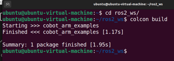
source ~/.bashrcRun the Node
In this section, we will finally run our node.
Here’s the general syntax for running a node:
ros2 run <package_name> <python_script_name>.pyHere’s a breakdown of the components:
- <package_name>: Replace this with the name of your ROS 2 package containing the Python script.
- <python_script_name>.py: Replace this with the name of your Python script file that contains the ROS 2 node.
Note that, you can use the tab button to autocomplete a partial command. For example, type the following and then press the TAB button on your keyboard.
ros2 run cobot_arm_examples minAfter autocompletion, the command looks like this:
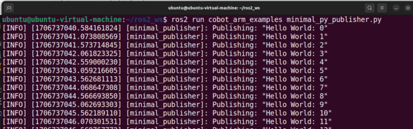
ros2 run cobot_arm_examples minimal_py_publisher.pyNow, press Enter.
Here is what the output looks like:
Open a new terminal window.
Let’s see a list of all currently active topics.
ros2 topic list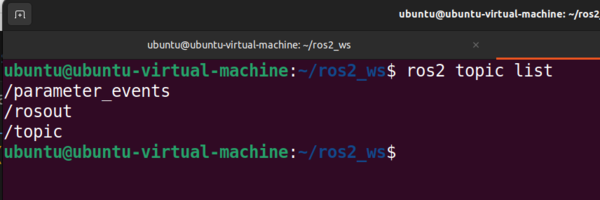
We see we have three active topics:
/parameter_events/rosout/topic/parameter_events and /rosout topics appear even when no nodes are actively running due to the presence of system-level components and the underlying architecture of the ROS 2 middleware.
The /parameter_events topic facilitates communication about parameter changes, and the /rosout topic provides a centralized way to access log messages generated by different nodes within the ROS 2 network.
/topic is the topic we created with our Python node. Let’s see what data is being published to this topic.
ros2 topic echo /topic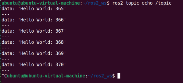
You can see the string message that is being published to this topic, including the counter integer we created in the Python script.
Press CTRL + C in the terminal to stop the output.
At what frequency is data being published to this topic?
ros2 topic hz /topicData is being published at 2Hz, or every 0.5 seconds.
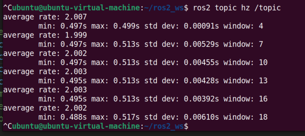
Press CTRL + C in the terminal to stop the output.
What type of data is being published to this topic, and how many nodes are publishing to this topic?
ros2 topic info /topic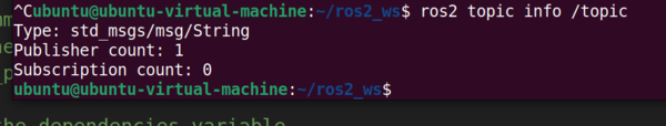
To get more detailed information about the topic, you could have typed:
ros2 topic info /topic --verboseWhat are the currently active nodes?
ros2 node list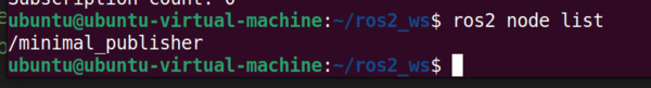
Let’s find out some more information about our node.
ros2 node info /minimal_publisher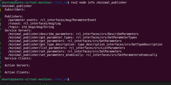
Close the Node
Now go back to the terminal where your minimal_py_publisher.py script is running and press CTRL + C to stop its execution.
To clear the terminal window, type:
clearCongratulations! You have written your first publisher in ROS 2.
In this example, you have written a publisher to publish a basic string message. On a real robot, you will write many different publishers that publish data that gets shared by the different components of a robot: strings, LIDAR scan readings, ultrasonic sensor readings, camera frames, 3D point cloud data, integers, float values, battery voltage readings, odometry data, and much more.
The code you wrote serves as a template for creating these more complex publishers. All publishers in ROS 2 are based on the basic framework as minimal_py_publisher.py.
That’s it. Keep building!

