Disclosure (#ad): As an Amazon Associate I earn from qualifying purchases.
Set Up the Hardware
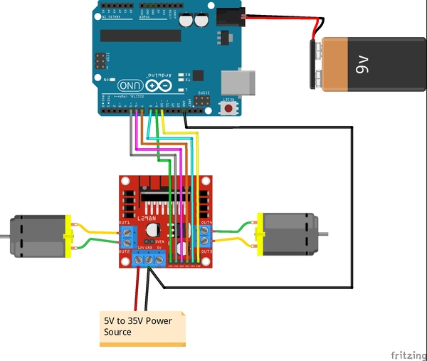
The first thing we need to do is set up the hardware. Below is the wiring diagram, and here is the pdf version so you can see the pin numbers better:
On my motors, the outer pins are the ones that drive the motors. These pins need to be connected to the L298N OUT1-OUT4 pins.
Remove the two black jumpers that are on the board that cover the ENA and ENB pins. Do not remove the other jumper that is near the power input pins.
Write the Code
Now let’s write the code. You will need to:
Load this code to your Arduino from your PC.
Remove the Arduino from your PC.
Turn on your Arduino using the 9V battery.
/*
 * Author: Automatic Addison
 * Website: https://automaticaddison.com
 * Description: Controls the speed and direction of two DC motors.
 */

// Motor A connections
const int enA = 9;
const int in1 = 5;
const int in2 = 6;

// Motor B connections
const int enB = 10;
const int in3 = 7;
const int in4 = 8;

// Set the speed (0 = off and 255 = max speed)
const int motorSpeed = 128;

void setup() {

  // Motor control pins are outputs
  pinMode(enA, OUTPUT);
  pinMode(enB, OUTPUT);
  pinMode(in1, OUTPUT);
  pinMode(in2, OUTPUT);
  pinMode(in3, OUTPUT);
  pinMode(in4, OUTPUT);

  // Turn off motors - Initial state
  digitalWrite(in1, LOW);
  digitalWrite(in2, LOW);
  digitalWrite(in3, LOW);
  digitalWrite(in4, LOW);

  // Set the motor speed
  analogWrite(enA, motorSpeed);
  analogWrite(enB, motorSpeed);
}

void loop() {

  // Go forwards
  go_forward();
  delay(3000);

  // Go backwards
  go_backwards();
  delay(3000);

  // Go right
  go_right();
  delay(3000);

  // Go left
  go_left();
  delay(3000);

  // Stop
  stop_all();
  delay(3000);
}

/*
 *  Forwards, backwards, right, left, stop.
 */
void go_forward() {
  digitalWrite(in1, HIGH);
  digitalWrite(in2, LOW);
  digitalWrite(in3, HIGH);
  digitalWrite(in4, LOW);
}
void go_backwards() {
  digitalWrite(in1, LOW);
  digitalWrite(in2, HIGH);
  digitalWrite(in3, LOW);
  digitalWrite(in4, HIGH);
}
void go_right() {
  digitalWrite(in1, HIGH);
  digitalWrite(in2, LOW);
  digitalWrite(in3, LOW);
  digitalWrite(in4, HIGH);
}
void go_left() {
  digitalWrite(in1, LOW);
  digitalWrite(in2, HIGH);
  digitalWrite(in3, HIGH);
  digitalWrite(in4, LOW);
}
void stop_all() {
  digitalWrite(in1, LOW);
  digitalWrite(in2, LOW);
  digitalWrite(in3, LOW);
  digitalWrite(in4, LOW);
}
Run the Code
When you run this code, you will see your motors move forwards, backwards, right turn, left turn, and then stop. If your motors don’t do this exact sequence, consider switching the position of the wire connections that both motors have to the L298N.
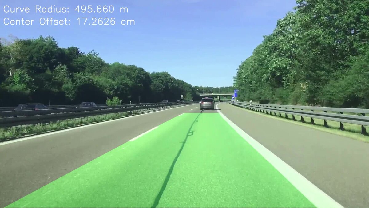
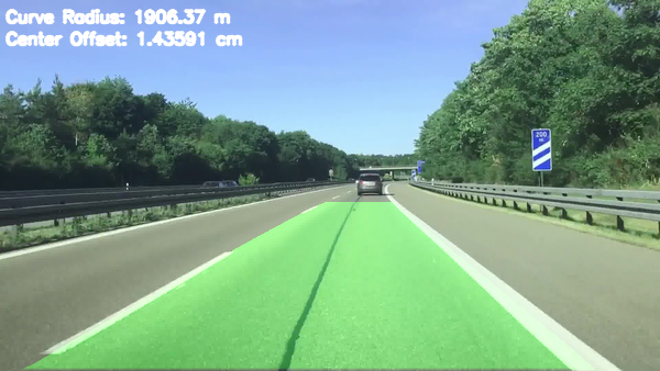
In this tutorial, we will go through the entire process, step by step, of how to detect lanes on a road in real time using the OpenCV computer vision library and Python. By the end of this tutorial, you will know how to build (from scratch) an application that can automatically detect lanes in a video stream from a front-facing camera mounted on a car. You’ll be able to generate this video below.
Our goal is to create a program that can read a video stream and output an annotated video that shows the following:
The current lane
The radius of curvature of the lane
The position of the vehicle relative to the middle of the lane
As you work through this tutorial, focus on the end goals I listed in the beginning. Don’t get bogged down in trying to understand every last detail of the math and the OpenCV operations we’ll use in our code (e.g. bitwise AND, Sobel edge detection algorithm etc.). Trust the developers at Intel who manage the OpenCV computer vision package.
We are trying to build products not publish research papers. Focus on the inputs, the outputs, and what the algorithm is supposed to do at a high level.
Get a working lane detection application up and running; and, at some later date when you want to add more complexity to your project or write a research paper, you can dive deeper under the hood to understand all the details.
Trying to understand every last detail is like trying to build your own database from scratch in order to start a website or taking a course on internal combustion engines to learn how to drive a car.
Let’s get started!
Find Some Videos and an Image
The first thing we need to do is find some videos and an image to serve as our test cases.
We want to download videos and an image that show a road with lanes from the perspective of a person driving a car.
I found some good candidates on Pixabay.com. Type “driving” or “lanes” in the video search on that website.
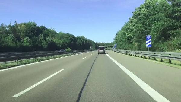
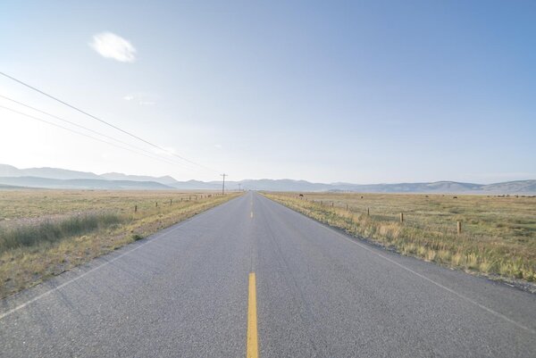
Here is an example of what a frame from one of your videos should look like. This frame is 600 pixels in width and 338 pixels in height:
Installation and Setup
We now need to make sure we have all the software packages installed. Check to see if you have OpenCV installed on your machine. If you are using Anaconda, you can type:
conda install -c conda-forge opencv
Alternatively, you can type:
pip install opencv-python
Make sure you have NumPy installed, a scientific computing library for Python.
If you’re using Anaconda, you can type:
conda install numpy
Alternatively, you can type:
pip install numpy
Install Matplotlib, a plotting library for Python.
For Anaconda users:
conda install -c conda-forge matplotlib
Otherwise, you can install like this:
pip install matplotlib
Python Code for Detection of Lane Lines in an Image
Before, we get started, I’ll share with you the full code you need to perform lane detection in an image. The two programs below are all you need to detect lane lines in an image.
You need to make sure that you save both programs below, edge_detection.py and lane.py in the same directory as the image.
edge_detection.py will be a collection of methods that helps isolate lane line edges and lane lines.
lane.py is where we will implement a Lane class that represents a lane on a road or highway.
Don’t be scared at how long the code appears. I always include a lot of comments in my code since I have the tendency to forget why I did what I did. I always want to be able to revisit my code at a later date and have a clear understanding what I did and why:
Here is edge_detection.py. Don’t worry, I’ll explain the code later in this post.
import cv2 # Import the OpenCV library to enable computer vision
import numpy as np # Import the NumPy scientific computing library

# Author: Addison Sears-Collins
# https://automaticaddison.com
# Description: A collection of methods to detect help with edge detection

def binary_array(array, thresh, value=0):
  """
  Return a 2D binary array (mask) in which all pixels are either 0 or 1

  :param array: NumPy 2D array that we want to convert to binary values
  :param thresh: Values used for thresholding (inclusive)
  :param value: Output value when between the supplied threshold
  :return: Binary 2D array...
           number of rows x number of columns =
           number of pixels from top to bottom x number of pixels from
             left to right
  """
  if value == 0:
    # Create an array of ones with the same shape and type as
    # the input 2D array.
    binary = np.ones_like(array)

  else:
    # Creates an array of zeros with the same shape and type as
    # the input 2D array.
    binary = np.zeros_like(array)
    value = 1

  # If value == 0, make all values in binary equal to 0 if the
  # corresponding value in the input array is between the threshold
  # (inclusive). Otherwise, the value remains as 1. Therefore, the pixels
  # with the high Sobel derivative values (i.e. sharp pixel intensity
  # discontinuities) will have 0 in the corresponding cell of binary.
  binary[(array >= thresh[0]) & (array <= thresh[1])] = value

  return binary

def blur_gaussian(channel, ksize=3):
  """
  Implementation for Gaussian blur to reduce noise and detail in the image

  :param image: 2D or 3D array to be blurred
  :param ksize: Size of the small matrix (i.e. kernel) used to blur
                i.e. number of rows and number of columns
  :return: Blurred 2D image
  """
  return cv2.GaussianBlur(channel, (ksize, ksize), 0)

def mag_thresh(image, sobel_kernel=3, thresh=(0, 255)):
  """
  Implementation of Sobel edge detection

  :param image: 2D or 3D array to be blurred
  :param sobel_kernel: Size of the small matrix (i.e. kernel)
                       i.e. number of rows and columns
  :return: Binary (black and white) 2D mask image
  """
  # Get the magnitude of the edges that are vertically aligned on the image
  sobelx = np.absolute(sobel(image, orient='x', sobel_kernel=sobel_kernel))

  # Get the magnitude of the edges that are horizontally aligned on the image
  sobely = np.absolute(sobel(image, orient='y', sobel_kernel=sobel_kernel))

  # Find areas of the image that have the strongest pixel intensity changes
  # in both the x and y directions. These have the strongest gradients and
  # represent the strongest edges in the image (i.e. potential lane lines)
  # mag is a 2D array .. number of rows x number of columns = number of pixels
  # from top to bottom x number of pixels from left to right
  mag = np.sqrt(sobelx ** 2 + sobely ** 2)

  # Return a 2D array that contains 0s and 1s
  return binary_array(mag, thresh)

def sobel(img_channel, orient='x', sobel_kernel=3):
  """
  Find edges that are aligned vertically and horizontally on the image

  :param img_channel: Channel from an image
  :param orient: Across which axis of the image are we detecting edges?
  :sobel_kernel: No. of rows and columns of the kernel (i.e. 3x3 small matrix)
  :return: Image with Sobel edge detection applied
  """
  # cv2.Sobel(input image, data type, prder of the derivative x, order of the
  # derivative y, small matrix used to calculate the derivative)
  if orient == 'x':
    # Will detect differences in pixel intensities going from
		# left to right on the image (i.e. edges that are vertically aligned)
    sobel = cv2.Sobel(img_channel, cv2.CV_64F, 1, 0, sobel_kernel)
  if orient == 'y':
    # Will detect differences in pixel intensities going from
    # top to bottom on the image (i.e. edges that are horizontally aligned)
    sobel = cv2.Sobel(img_channel, cv2.CV_64F, 0, 1, sobel_kernel)

  return sobel

def threshold(channel, thresh=(128,255), thresh_type=cv2.THRESH_BINARY):
  """
  Apply a threshold to the input channel

  :param channel: 2D array of the channel data of an image/video frame
  :param thresh: 2D tuple of min and max threshold values
  :param thresh_type: The technique of the threshold to apply
  :return: Two outputs are returned:
             ret: Threshold that was used
   	         thresholded_image: 2D thresholded data.
  """
  # If pixel intensity is greater than thresh[0], make that value
  # white (255), else set it to black (0)
  return cv2.threshold(channel, thresh[0], thresh[1], thresh_type)
Here is lane.py.
import cv2 # Import the OpenCV library to enable computer vision
import numpy as np # Import the NumPy scientific computing library
import edge_detection as edge # Handles the detection of lane lines
import matplotlib.pyplot as plt # Used for plotting and error checking
# Author: Addison Sears-Collins
# https://automaticaddison.com
# Description: Implementation of the Lane class
filename = 'original_lane_detection_5.jpg'
class Lane:
"""
Represents a lane on a road.
"""
def __init__(self, orig_frame):
"""
Default constructor
:param orig_frame: Original camera image (i.e. frame)
"""
self.orig_frame = orig_frame
# This will hold an image with the lane lines
self.lane_line_markings = None
# This will hold the image after perspective transformation
self.warped_frame = None
self.transformation_matrix = None
self.inv_transformation_matrix = None
# (Width, Height) of the original video frame (or image)
self.orig_image_size = self.orig_frame.shape[::-1][1:]
width = self.orig_image_size[0]
height = self.orig_image_size[1]
self.width = width
self.height = height
# Four corners of the trapezoid-shaped region of interest
# You need to find these corners manually.
self.roi_points = np.float32([
(274,184), # Top-left corner
(0, 337), # Bottom-left corner
(575,337), # Bottom-right corner
(371,184) # Top-right corner
])
# The desired corner locations of the region of interest
# after we perform perspective transformation.
# Assume image width of 600, padding == 150.
self.padding = int(0.25 * width) # padding from side of the image in pixels
self.desired_roi_points = np.float32([
[self.padding, 0], # Top-left corner
[self.padding, self.orig_image_size[1]], # Bottom-left corner
[self.orig_image_size[
0]-self.padding, self.orig_image_size[1]], # Bottom-right corner
[self.orig_image_size[0]-self.padding, 0] # Top-right corner
])
# Histogram that shows the white pixel peaks for lane line detection
self.histogram = None
# Sliding window parameters
self.no_of_windows = 10
self.margin = int((1/12) * width) # Window width is +/- margin
self.minpix = int((1/24) * width) # Min no. of pixels to recenter window
# Best fit polynomial lines for left line and right line of the lane
self.left_fit = None
self.right_fit = None
self.left_lane_inds = None
self.right_lane_inds = None
self.ploty = None
self.left_fitx = None
self.right_fitx = None
self.leftx = None
self.rightx = None
self.lefty = None
self.righty = None
# Pixel parameters for x and y dimensions
self.YM_PER_PIX = 10.0 / 1000 # meters per pixel in y dimension
self.XM_PER_PIX = 3.7 / 781 # meters per pixel in x dimension
# Radii of curvature and offset
self.left_curvem = None
self.right_curvem = None
self.center_offset = None
def calculate_car_position(self, print_to_terminal=False):
"""
Calculate the position of the car relative to the center
:param: print_to_terminal Display data to console if True
:return: Offset from the center of the lane
"""
# Assume the camera is centered in the image.
# Get position of car in centimeters
car_location = self.orig_frame.shape[1] / 2
# Fine the x coordinate of the lane line bottom
height = self.orig_frame.shape[0]
bottom_left = self.left_fit[0]*height**2 + self.left_fit[
1]*height + self.left_fit[2]
bottom_right = self.right_fit[0]*height**2 + self.right_fit[
1]*height + self.right_fit[2]
center_lane = (bottom_right - bottom_left)/2 + bottom_left
center_offset = (np.abs(car_location) - np.abs(
center_lane)) * self.XM_PER_PIX * 100
if print_to_terminal == True:
print(str(center_offset) + 'cm')
self.center_offset = center_offset
return center_offset
def calculate_curvature(self, print_to_terminal=False):
"""
Calculate the road curvature in meters.
:param: print_to_terminal Display data to console if True
:return: Radii of curvature
"""
# Set the y-value where we want to calculate the road curvature.
# Select the maximum y-value, which is the bottom of the frame.
y_eval = np.max(self.ploty)
# Fit polynomial curves to the real world environment
left_fit_cr = np.polyfit(self.lefty * self.YM_PER_PIX, self.leftx * (
self.XM_PER_PIX), 2)
right_fit_cr = np.polyfit(self.righty * self.YM_PER_PIX, self.rightx * (
self.XM_PER_PIX), 2)
# Calculate the radii of curvature
left_curvem = ((1 + (2*left_fit_cr[0]*y_eval*self.YM_PER_PIX + left_fit_cr[
1])**2)**1.5) / np.absolute(2*left_fit_cr[0])
right_curvem = ((1 + (2*right_fit_cr[
0]*y_eval*self.YM_PER_PIX + right_fit_cr[
1])**2)**1.5) / np.absolute(2*right_fit_cr[0])
# Display on terminal window
if print_to_terminal == True:
print(left_curvem, 'm', right_curvem, 'm')
self.left_curvem = left_curvem
self.right_curvem = right_curvem
return left_curvem, right_curvem
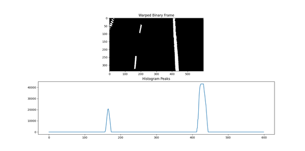
def calculate_histogram(self,frame=None,plot=True):
"""
Calculate the image histogram to find peaks in white pixel count
:param frame: The warped image
:param plot: Create a plot if True
"""
if frame is None:
frame = self.warped_frame
# Generate the histogram
self.histogram = np.sum(frame[int(
frame.shape[0]/2):,:], axis=0)
if plot == True:
# Draw both the image and the histogram
figure, (ax1, ax2) = plt.subplots(2,1) # 2 row, 1 columns
figure.set_size_inches(10, 5)
ax1.imshow(frame, cmap='gray')
ax1.set_title("Warped Binary Frame")
ax2.plot(self.histogram)
ax2.set_title("Histogram Peaks")
plt.show()
return self.histogram
def display_curvature_offset(self, frame=None, plot=False):
"""
Display curvature and offset statistics on the image
:param: plot Display the plot if True
:return: Image with lane lines and curvature
"""
image_copy = None
if frame is None:
image_copy = self.orig_frame.copy()
else:
image_copy = frame
cv2.putText(image_copy,'Curve Radius: '+str((
self.left_curvem+self.right_curvem)/2)[:7]+' m', (int((
5/600)*self.width), int((
20/338)*self.height)), cv2.FONT_HERSHEY_SIMPLEX, (float((
0.5/600)*self.width)),(
255,255,255),2,cv2.LINE_AA)
cv2.putText(image_copy,'Center Offset: '+str(
self.center_offset)[:7]+' cm', (int((
5/600)*self.width), int((
40/338)*self.height)), cv2.FONT_HERSHEY_SIMPLEX, (float((
0.5/600)*self.width)),(
255,255,255),2,cv2.LINE_AA)
if plot==True:
cv2.imshow("Image with Curvature and Offset", image_copy)
return image_copy
def get_lane_line_previous_window(self, left_fit, right_fit, plot=False):
"""
Use the lane line from the previous sliding window to get the parameters
for the polynomial line for filling in the lane line
:param: left_fit Polynomial function of the left lane line
:param: right_fit Polynomial function of the right lane line
:param: plot To display an image or not
"""
# margin is a sliding window parameter
margin = self.margin
# Find the x and y coordinates of all the nonzero
# (i.e. white) pixels in the frame.
nonzero = self.warped_frame.nonzero()
nonzeroy = np.array(nonzero[0])
nonzerox = np.array(nonzero[1])
# Store left and right lane pixel indices
left_lane_inds = ((nonzerox > (left_fit[0]*(
nonzeroy**2) + left_fit[1]*nonzeroy + left_fit[2] - margin)) & (
nonzerox < (left_fit[0]*(
nonzeroy**2) + left_fit[1]*nonzeroy + left_fit[2] + margin)))
right_lane_inds = ((nonzerox > (right_fit[0]*(
nonzeroy**2) + right_fit[1]*nonzeroy + right_fit[2] - margin)) & (
nonzerox < (right_fit[0]*(
nonzeroy**2) + right_fit[1]*nonzeroy + right_fit[2] + margin)))
self.left_lane_inds = left_lane_inds
self.right_lane_inds = right_lane_inds
# Get the left and right lane line pixel locations
leftx = nonzerox[left_lane_inds]
lefty = nonzeroy[left_lane_inds]
rightx = nonzerox[right_lane_inds]
righty = nonzeroy[right_lane_inds]
self.leftx = leftx
self.rightx = rightx
self.lefty = lefty
self.righty = righty
# Fit a second order polynomial curve to each lane line
left_fit = np.polyfit(lefty, leftx, 2)
right_fit = np.polyfit(righty, rightx, 2)
self.left_fit = left_fit
self.right_fit = right_fit
# Create the x and y values to plot on the image
ploty = np.linspace(
0, self.warped_frame.shape[0]-1, self.warped_frame.shape[0])
left_fitx = left_fit[0]*ploty**2 + left_fit[1]*ploty + left_fit[2]
right_fitx = right_fit[0]*ploty**2 + right_fit[1]*ploty + right_fit[2]
self.ploty = ploty
self.left_fitx = left_fitx
self.right_fitx = right_fitx
if plot==True:
# Generate images to draw on
out_img = np.dstack((self.warped_frame, self.warped_frame, (
self.warped_frame)))*255
window_img = np.zeros_like(out_img)
# Add color to the left and right line pixels
out_img[nonzeroy[left_lane_inds], nonzerox[left_lane_inds]] = [255, 0, 0]
out_img[nonzeroy[right_lane_inds], nonzerox[right_lane_inds]] = [
0, 0, 255]
# Create a polygon to show the search window area, and recast
# the x and y points into a usable format for cv2.fillPoly()
margin = self.margin
left_line_window1 = np.array([np.transpose(np.vstack([
left_fitx-margin, ploty]))])
left_line_window2 = np.array([np.flipud(np.transpose(np.vstack([
left_fitx+margin, ploty])))])
left_line_pts = np.hstack((left_line_window1, left_line_window2))
right_line_window1 = np.array([np.transpose(np.vstack([
right_fitx-margin, ploty]))])
right_line_window2 = np.array([np.flipud(np.transpose(np.vstack([
right_fitx+margin, ploty])))])
right_line_pts = np.hstack((right_line_window1, right_line_window2))
# Draw the lane onto the warped blank image
cv2.fillPoly(window_img, np.int_([left_line_pts]), (0,255, 0))
cv2.fillPoly(window_img, np.int_([right_line_pts]), (0,255, 0))
result = cv2.addWeighted(out_img, 1, window_img, 0.3, 0)
# Plot the figures
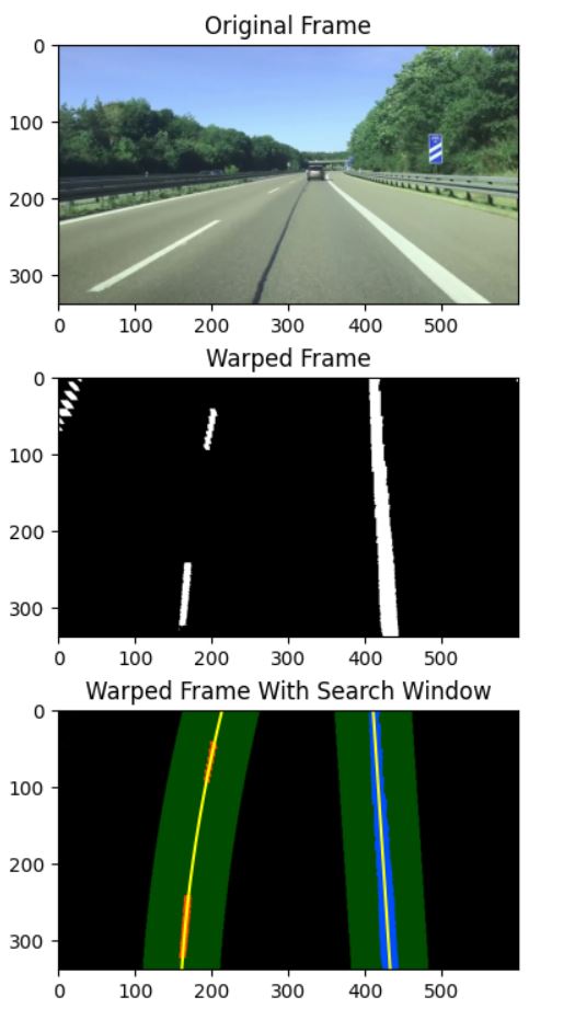
figure, (ax1, ax2, ax3) = plt.subplots(3,1) # 3 rows, 1 column
figure.set_size_inches(10, 10)
figure.tight_layout(pad=3.0)
ax1.imshow(cv2.cvtColor(self.orig_frame, cv2.COLOR_BGR2RGB))
ax2.imshow(self.warped_frame, cmap='gray')
ax3.imshow(result)
ax3.plot(left_fitx, ploty, color='yellow')
ax3.plot(right_fitx, ploty, color='yellow')
ax1.set_title("Original Frame")
ax2.set_title("Warped Frame")
ax3.set_title("Warped Frame With Search Window")
plt.show()
def get_lane_line_indices_sliding_windows(self, plot=False):
"""
Get the indices of the lane line pixels using the
sliding windows technique.
:param: plot Show plot or not
:return: Best fit lines for the left and right lines of the current lane
"""
# Sliding window width is +/- margin
margin = self.margin
frame_sliding_window = self.warped_frame.copy()
# Set the height of the sliding windows
window_height = np.int(self.warped_frame.shape[0]/self.no_of_windows)
# Find the x and y coordinates of all the nonzero
# (i.e. white) pixels in the frame.
nonzero = self.warped_frame.nonzero()
nonzeroy = np.array(nonzero[0])
nonzerox = np.array(nonzero[1])
# Store the pixel indices for the left and right lane lines
left_lane_inds = []
right_lane_inds = []
# Current positions for pixel indices for each window,
# which we will continue to update
leftx_base, rightx_base = self.histogram_peak()
leftx_current = leftx_base
rightx_current = rightx_base
# Go through one window at a time
no_of_windows = self.no_of_windows
for window in range(no_of_windows):
# Identify window boundaries in x and y (and right and left)
win_y_low = self.warped_frame.shape[0] - (window + 1) * window_height
win_y_high = self.warped_frame.shape[0] - window * window_height
win_xleft_low = leftx_current - margin
win_xleft_high = leftx_current + margin
win_xright_low = rightx_current - margin
win_xright_high = rightx_current + margin
cv2.rectangle(frame_sliding_window,(win_xleft_low,win_y_low),(
win_xleft_high,win_y_high), (255,255,255), 2)
cv2.rectangle(frame_sliding_window,(win_xright_low,win_y_low),(
win_xright_high,win_y_high), (255,255,255), 2)
# Identify the nonzero pixels in x and y within the window
good_left_inds = ((nonzeroy >= win_y_low) & (nonzeroy < win_y_high) &
(nonzerox >= win_xleft_low) & (
nonzerox < win_xleft_high)).nonzero()[0]
good_right_inds = ((nonzeroy >= win_y_low) & (nonzeroy < win_y_high) &
(nonzerox >= win_xright_low) & (
nonzerox < win_xright_high)).nonzero()[0]
# Append these indices to the lists
left_lane_inds.append(good_left_inds)
right_lane_inds.append(good_right_inds)
# If you found > minpix pixels, recenter next window on mean position
minpix = self.minpix
if len(good_left_inds) > minpix:
leftx_current = np.int(np.mean(nonzerox[good_left_inds]))
if len(good_right_inds) > minpix:
rightx_current = np.int(np.mean(nonzerox[good_right_inds]))
# Concatenate the arrays of indices
left_lane_inds = np.concatenate(left_lane_inds)
right_lane_inds = np.concatenate(right_lane_inds)
# Extract the pixel coordinates for the left and right lane lines
leftx = nonzerox[left_lane_inds]
lefty = nonzeroy[left_lane_inds]
rightx = nonzerox[right_lane_inds]
righty = nonzeroy[right_lane_inds]
# Fit a second order polynomial curve to the pixel coordinates for
# the left and right lane lines
left_fit = np.polyfit(lefty, leftx, 2)
right_fit = np.polyfit(righty, rightx, 2)
self.left_fit = left_fit
self.right_fit = right_fit
if plot==True:
# Create the x and y values to plot on the image
ploty = np.linspace(
0, frame_sliding_window.shape[0]-1, frame_sliding_window.shape[0])
left_fitx = left_fit[0]*ploty**2 + left_fit[1]*ploty + left_fit[2]
right_fitx = right_fit[0]*ploty**2 + right_fit[1]*ploty + right_fit[2]
# Generate an image to visualize the result
out_img = np.dstack((
frame_sliding_window, frame_sliding_window, (
frame_sliding_window))) * 255
# Add color to the left line pixels and right line pixels
out_img[nonzeroy[left_lane_inds], nonzerox[left_lane_inds]] = [255, 0, 0]
out_img[nonzeroy[right_lane_inds], nonzerox[right_lane_inds]] = [
0, 0, 255]
# Plot the figure with the sliding windows
figure, (ax1, ax2, ax3) = plt.subplots(3,1) # 3 rows, 1 column
figure.set_size_inches(10, 10)
figure.tight_layout(pad=3.0)
ax1.imshow(cv2.cvtColor(self.orig_frame, cv2.COLOR_BGR2RGB))
ax2.imshow(frame_sliding_window, cmap='gray')
ax3.imshow(out_img)
ax3.plot(left_fitx, ploty, color='yellow')
ax3.plot(right_fitx, ploty, color='yellow')
ax1.set_title("Original Frame")
ax2.set_title("Warped Frame with Sliding Windows")
ax3.set_title("Detected Lane Lines with Sliding Windows")
plt.show()
return self.left_fit, self.right_fit
def get_line_markings(self, frame=None):
"""
Isolates lane lines.
:param frame: The camera frame that contains the lanes we want to detect
:return: Binary (i.e. black and white) image containing the lane lines.
"""
if frame is None:
frame = self.orig_frame
# Convert the video frame from BGR (blue, green, red)
# color space to HLS (hue, saturation, lightness).
hls = cv2.cvtColor(frame, cv2.COLOR_BGR2HLS)
################### Isolate possible lane line edges ######################
# Perform Sobel edge detection on the L (lightness) channel of
# the image to detect sharp discontinuities in the pixel intensities
# along the x and y axis of the video frame.
# sxbinary is a matrix full of 0s (black) and 255 (white) intensity values
# Relatively light pixels get made white. Dark pixels get made black.
_, sxbinary = edge.threshold(hls[:, :, 1], thresh=(120, 255))
sxbinary = edge.blur_gaussian(sxbinary, ksize=3) # Reduce noise
# 1s will be in the cells with the highest Sobel derivative values
# (i.e. strongest lane line edges)
sxbinary = edge.mag_thresh(sxbinary, sobel_kernel=3, thresh=(110, 255))
######################## Isolate possible lane lines ######################
# Perform binary thresholding on the S (saturation) channel
# of the video frame. A high saturation value means the hue color is pure.
# We expect lane lines to be nice, pure colors (i.e. solid white, yellow)
# and have high saturation channel values.
# s_binary is matrix full of 0s (black) and 255 (white) intensity values
# White in the regions with the purest hue colors (e.g. >80...play with
# this value for best results).
s_channel = hls[:, :, 2] # use only the saturation channel data
_, s_binary = edge.threshold(s_channel, (80, 255))
# Perform binary thresholding on the R (red) channel of the
# original BGR video frame.
# r_thresh is a matrix full of 0s (black) and 255 (white) intensity values
# White in the regions with the richest red channel values (e.g. >120).
# Remember, pure white is bgr(255, 255, 255).
# Pure yellow is bgr(0, 255, 255). Both have high red channel values.
_, r_thresh = edge.threshold(frame[:, :, 2], thresh=(120, 255))
# Lane lines should be pure in color and have high red channel values
# Bitwise AND operation to reduce noise and black-out any pixels that
# don't appear to be nice, pure, solid colors (like white or yellow lane
# lines.)
rs_binary = cv2.bitwise_and(s_binary, r_thresh)
### Combine the possible lane lines with the possible lane line edges #####
# If you show rs_binary visually, you'll see that it is not that different
# from this return value. The edges of lane lines are thin lines of pixels.
self.lane_line_markings = cv2.bitwise_or(rs_binary, sxbinary.astype(
np.uint8))
return self.lane_line_markings
def histogram_peak(self):
"""
Get the left and right peak of the histogram
Return the x coordinate of the left histogram peak and the right histogram
peak.
"""
midpoint = np.int(self.histogram.shape[0]/2)
leftx_base = np.argmax(self.histogram[:midpoint])
rightx_base = np.argmax(self.histogram[midpoint:]) + midpoint
# (x coordinate of left peak, x coordinate of right peak)
return leftx_base, rightx_base
def overlay_lane_lines(self, plot=False):
"""
Overlay lane lines on the original frame
:param: Plot the lane lines if True
:return: Lane with overlay
"""
# Generate an image to draw the lane lines on
warp_zero = np.zeros_like(self.warped_frame).astype(np.uint8)
color_warp = np.dstack((warp_zero, warp_zero, warp_zero))
# Recast the x and y points into usable format for cv2.fillPoly()
pts_left = np.array([np.transpose(np.vstack([
self.left_fitx, self.ploty]))])
pts_right = np.array([np.flipud(np.transpose(np.vstack([
self.right_fitx, self.ploty])))])
pts = np.hstack((pts_left, pts_right))
# Draw lane on the warped blank image
cv2.fillPoly(color_warp, np.int_([pts]), (0,255, 0))
# Warp the blank back to original image space using inverse perspective
# matrix (Minv)
newwarp = cv2.warpPerspective(color_warp, self.inv_transformation_matrix, (
self.orig_frame.shape[
1], self.orig_frame.shape[0]))
# Combine the result with the original image
result = cv2.addWeighted(self.orig_frame, 1, newwarp, 0.3, 0)
if plot==True:
# Plot the figures
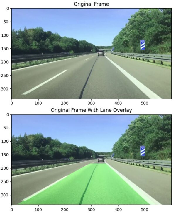
figure, (ax1, ax2) = plt.subplots(2,1) # 2 rows, 1 column
figure.set_size_inches(10, 10)
figure.tight_layout(pad=3.0)
ax1.imshow(cv2.cvtColor(self.orig_frame, cv2.COLOR_BGR2RGB))
ax2.imshow(cv2.cvtColor(result, cv2.COLOR_BGR2RGB))
ax1.set_title("Original Frame")
ax2.set_title("Original Frame With Lane Overlay")
plt.show()
return result
def perspective_transform(self, frame=None, plot=False):
"""
Perform the perspective transform.
:param: frame Current frame
:param: plot Plot the warped image if True
:return: Bird's eye view of the current lane
"""
if frame is None:
frame = self.lane_line_markings
# Calculate the transformation matrix
self.transformation_matrix = cv2.getPerspectiveTransform(
self.roi_points, self.desired_roi_points)
# Calculate the inverse transformation matrix
self.inv_transformation_matrix = cv2.getPerspectiveTransform(
self.desired_roi_points, self.roi_points)
# Perform the transform using the transformation matrix
self.warped_frame = cv2.warpPerspective(
frame, self.transformation_matrix, self.orig_image_size, flags=(
cv2.INTER_LINEAR))
# Convert image to binary
(thresh, binary_warped) = cv2.threshold(
self.warped_frame, 127, 255, cv2.THRESH_BINARY)
self.warped_frame = binary_warped
# Display the perspective transformed (i.e. warped) frame
if plot == True:
warped_copy = self.warped_frame.copy()
warped_plot = cv2.polylines(warped_copy, np.int32([
self.desired_roi_points]), True, (147,20,255), 3)
# Display the image
while(1):
cv2.imshow('Warped Image', warped_plot)
# Press any key to stop
if cv2.waitKey(0):
break
cv2.destroyAllWindows()
return self.warped_frame
def plot_roi(self, frame=None, plot=False):
"""
Plot the region of interest on an image.
:param: frame The current image frame
:param: plot Plot the roi image if True
"""
if plot == False:
return
if frame is None:
frame = self.orig_frame.copy()
# Overlay trapezoid on the frame
this_image = cv2.polylines(frame, np.int32([
self.roi_points]), True, (147,20,255), 3)
# Display the image
while(1):
cv2.imshow('ROI Image', this_image)
# Press any key to stop
if cv2.waitKey(0):
break
cv2.destroyAllWindows()
def main():
# Load a frame (or image)
original_frame = cv2.imread(filename)
# Create a Lane object
lane_obj = Lane(orig_frame=original_frame)
# Perform thresholding to isolate lane lines
lane_line_markings = lane_obj.get_line_markings()
# Plot the region of interest on the image
lane_obj.plot_roi(plot=False)
# Perform the perspective transform to generate a bird's eye view
# If Plot == True, show image with new region of interest
warped_frame = lane_obj.perspective_transform(plot=False)
# Generate the image histogram to serve as a starting point
# for finding lane line pixels
histogram = lane_obj.calculate_histogram(plot=False)
# Find lane line pixels using the sliding window method
left_fit, right_fit = lane_obj.get_lane_line_indices_sliding_windows(
plot=False)
# Fill in the lane line
lane_obj.get_lane_line_previous_window(left_fit, right_fit, plot=False)
# Overlay lines on the original frame
frame_with_lane_lines = lane_obj.overlay_lane_lines(plot=False)
# Calculate lane line curvature (left and right lane lines)
lane_obj.calculate_curvature(print_to_terminal=False)
# Calculate center offset
lane_obj.calculate_car_position(print_to_terminal=False)
# Display curvature and center offset on image
frame_with_lane_lines2 = lane_obj.display_curvature_offset(
frame=frame_with_lane_lines, plot=True)
# Create the output file name by removing the '.jpg' part
size = len(filename)
new_filename = filename[:size - 4]
new_filename = new_filename + '_thresholded.jpg'
# Save the new image in the working directory
#cv2.imwrite(new_filename, lane_line_markings)
# Display the image
#cv2.imshow("Image", lane_line_markings)
# Display the window until any key is pressed
cv2.waitKey(0)
# Close all windows
cv2.destroyAllWindows()
main()
Now that you have all the code to detect lane lines in an image, let’s explain what each piece of the code does.
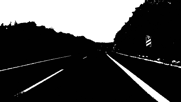
Isolate Pixels That Could Represent Lane Lines
The first part of the lane detection process is to apply thresholding (I’ll explain what this term means in a second) to each video frame so that we can eliminate things that make it difficult to detect lane lines. By applying thresholding, we can isolate the pixels that represent lane lines.
Glare from the sun, shadows, car headlights, and road surface changes can all make it difficult to find lanes in a video frame or image.
What does thresholding mean? Basic thresholding involves replacing each pixel in a video frame with a black pixel if the intensity of that pixel is less than some constant, or a white pixel if the intensity of that pixel is greater than some constant. The end result is a binary (black and white) image of the road. A binary image is one in which each pixel is either 1 (white) or 0 (black).
There are a lot of ways to represent colors in an image. If you’ve ever used a program like Microsoft Paint or Adobe Photoshop, you know that one way to represent a color is by using the RGB color space (in OpenCV it is BGR instead of RGB), where every color is a mixture of three colors, red, green, and blue. You can play around with the RGB color space here at this website.
The HLS color space is better than the BGR color space for detecting image issues due to lighting, such as shadows, glare from the sun, headlights, etc. We want to eliminate all these things to make it easier to detect lane lines. For this reason, we use the HLS color space, which divides all colors into hue, saturation, and lightness values.
If you want to play around with the HLS color space, there are a lot of HLS color picker websites to choose from if you do a Google search.
2. Perform Sobel edge detection on the L (lightness) channel of the image to detect sharp discontinuities in the pixel intensities along the x and y axis of the video frame.
Sharp changes in intensity from one pixel to a neighboring pixel means that an edge is likely present. We want to detect the strongest edges in the image so that we can isolate potential lane line edges.
3. Perform binary thresholding on the S (saturation) channel of the video frame.
Doing this helps to eliminate dull road colors.
A high saturation value means the hue color is pure. We expect lane lines to be nice, pure colors, such as solid white and solid yellow. Both solid white and solid yellow, have high saturation channel values.
Binary thresholding generates an image that is full of 0s (black) and 255 (white) intensity values. Pixels with high saturation values (e.g. > 80 on a scale from 0 to 255) will be set to white, while everything else will be set to black.
Feel free to play around with that threshold value. I set it to 80, but you can set it to another number, and see if you get better results.
4. Perform binary thresholding on the R (red) channel of the original BGR video frame.
This step helps extract the yellow and white color values, which are the typical colors of lane lines.
Remember, pure white is bgr(255, 255, 255). Pure yellow is bgr(0, 255, 255). Both have high red channel values.
To generate our binary image at this stage, pixels that have rich red channel values (e.g. > 120 on a scale from 0 to 255) will be set to white. All other pixels will be set to black.
5. Perform the bitwise AND operation to reduce noise in the image caused by shadows and variations in the road color.
Lane lines should be pure in color and have high red channel values. The bitwise AND operation reduces noise and blacks-out any pixels that don’t appear to be nice, pure, solid colors (like white or yellow lane lines.)
The get_line_markings(self, frame=None) method in lane.py performs all the steps I have mentioned above.
If you uncomment this line below, you will see the output:
cv2.imshow("Image", lane_line_markings)
To see the output, you run this command from within the directory with your test image and the lane.py and edge_detection.py program.
python lane.py
For best results, play around with this line on the lane.py program. Move the 80 value up or down, and see what results you get.
Now that we know how to isolate lane lines in an image, let’s continue on to the next step of the lane detection process.
Apply Perspective Transformation to Get a Bird’s Eye View
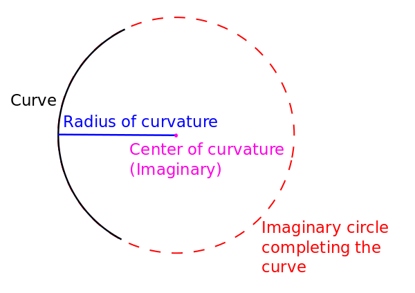
We now know how to isolate lane lines in an image, but we still have some problems. Remember that one of the goals of this project was to calculate the radius of curvature of the road lane. Calculating the radius of curvature will enable us to know which direction the road is turning. But we can’t do this yet at this stage due to the perspective of the camera. Let me explain.
Why We Need to Do Perspective Transformation
Imagine you’re a bird. You’re flying high above the road lanes below. From a birds-eye view, the lines on either side of the lane look like they are parallel.
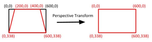
However, from the perspective of the camera mounted on a car below, the lane lines make a trapezoid-like shape. We can’t properly calculate the radius of curvature of the lane because, from the camera’s perspective, the lane width appears to decrease the farther away you get from the car.
In fact, way out on the horizon, the lane lines appear to converge to a point (known in computer vision jargon as vanishing point). You can see this effect in the image below:
The camera’s perspective is therefore not an accurate representation of what is going on in the real world. We need to fix this so that we can calculate the curvature of the land and the road (which will later help us when we want to steer the car appropriately).
How Perspective Transformation Works
Fortunately, OpenCV has methods that help us perform perspective transformation (i.e. projective transformation or projective geometry). These methods warp the camera’s perspective into a birds-eye view (i.e. aerial view) perspective.
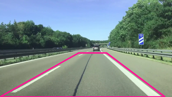
For the first step of perspective transformation, we need to identify a region of interest (ROI). This step helps remove parts of the image we’re not interested in. We are only interested in the lane segment that is immediately in front of the car.
You can run lane.py from the previous section. With the image displayed, hover your cursor over the image and find the four key corners of the trapezoid.
Write these corners down. These will be the roi_points (roi = region of interest) for the lane. In the code (which I’ll show below), these points appear in the __init__ constructor of the Lane class. They are stored in the self.roi_points variable.
In the following line of code in lane.py, change the parameter value from False to True so that the region of interest image will appear.
lane_obj.plot_roi(plot=True)
Run lane.py
python lane.py
Here is an example ROI output:
You can see that the ROI is the shape of a trapezoid, with four distinct corners.
Now that we have the region of interest, we use OpenCV’s getPerspectiveTransform and warpPerspectivemethods to transform the trapezoid-like perspective into a rectangle-like perspective.
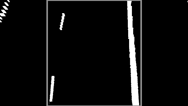
Change the parameter value in this line of code in lane.py from False to True.
Here is an example of an image after this process. You can see how the perspective is now from a birds-eye view. The ROI lines are now parallel to the sides of the image, making it easier to calculate the curvature of the road and the lane.
Identify Lane Line Pixels
We now need to identify the pixels on the warped image that make up lane lines. Looking at the warped image, we can see that white pixels represent pieces of the lane lines.
We start lane line pixel detection by generating a histogram to locate areas of the image that have high concentrations of white pixels.
Ideally, when we draw the histogram, we will have two peaks. There will be a left peak and a right peak, corresponding to the left lane line and the right lane line, respectively.
In lane.py, make sure to change the parameter value in this line of code (inside the main() method) from False to True so that the histogram will display.
The next step is to use a sliding window technique where we start at the bottom of the image and scan all the way to the top of the image. Each time we search within a sliding window, we add potential lane line pixels to a list. If we have enough lane line pixels in a window, the mean position of these pixels becomes the center of the next sliding window.
Once we have identified the pixels that correspond to the left and right lane lines, we draw a polynomial best-fit line through the pixels. This line represents our best estimate of the lane lines.
In this line of code, change the value from False to True.
If you run the code on different videos, you may see a warning that says “RankWarning: Polyfit may be poorly conditioned”. If you see this warning, try playing around with the dimensions of the region of interest as well as the thresholds.
You can also play with the length of the moving averages. I used a 10-frame moving average, but you can try another value like 5 or 25:
if len(prev_left_fit2) > 10:
Using an exponential moving average instead of a simple moving average might yield better results as well.
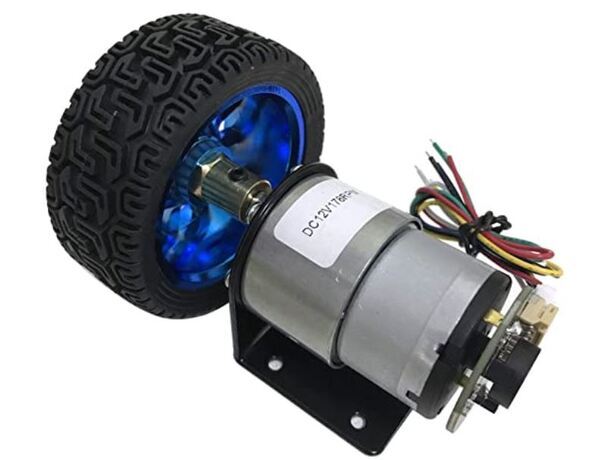
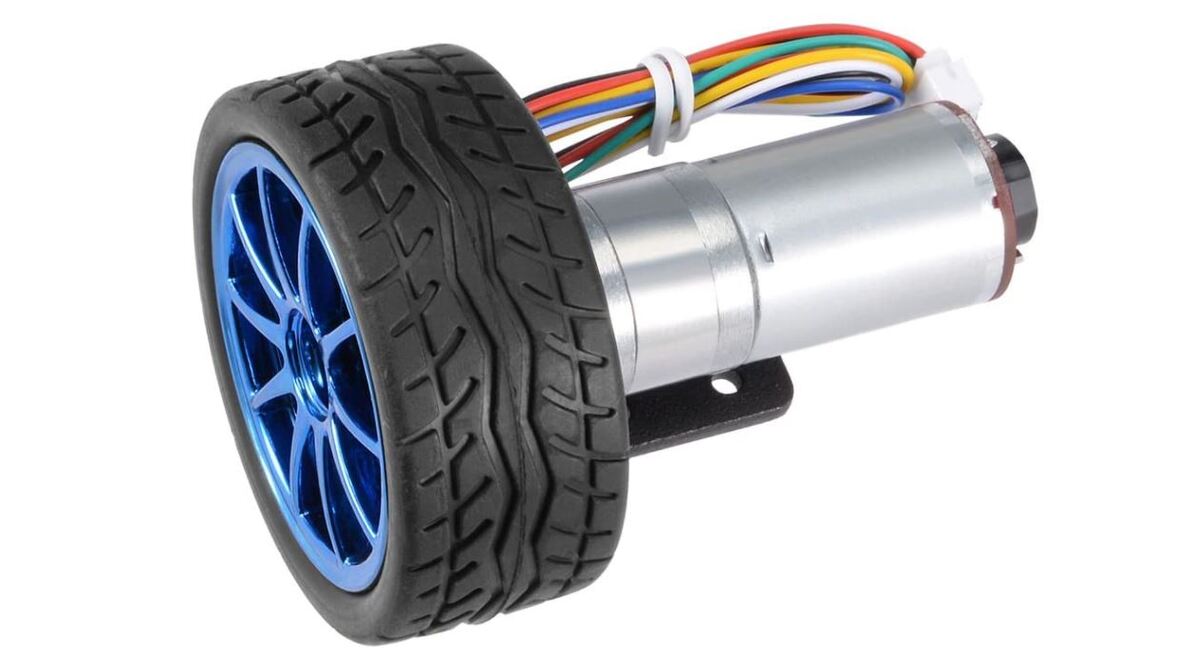
In this tutorial, we learn how to calculate the angular velocity (magnitude and direction of rotation in radians per second) of a DC motor with a built-in encoder.
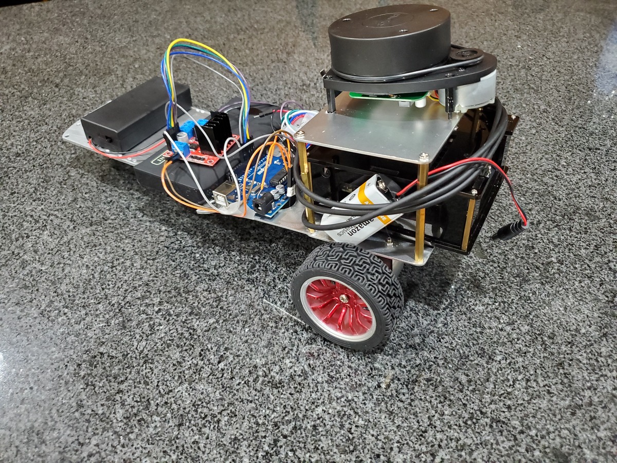
Here is the motor we will work with, but you can use any motor that looks like this one.
Real-World Applications
Knowing the angular velocity of wheels on a robot helps us calculate how fast the robot is moving (i.e. speed) as well as the distance a robot has traveled in a given unit of time. This information is important for helping us determine where a robot is in a particular environment (i.e. odometry).
Prerequisites
You have the Arduino IDE (Integrated Development Environment) installed on your PC (Windows, MacOS, or Linux).
Self-Balancing Car Kit (which includes everything above and more…Elegoo and Osoyoo are good brands you can find on Amazon.com)
Disclosure (#ad): As an Amazon Associate I earn from qualifying purchases.
Set Up the Hardware
The first thing we need to do is set up the hardware.
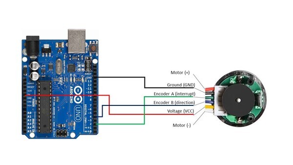
Here is the wiring diagram:
The Ground pin of the motor connects to GND of the Arduino.
Encoder A (sometimes labeled C1) of the motor connects to pin 2 of the Arduino. Pin 2 of the Arduino will record every time there is a rising digital signal from Encoder A.
Encoder B (sometimes labeled C2) of the motor connects to pin 4 of the Arduino. The signal that is read off pin 4 on the Arduino will determine if the motor is moving forward or in reverse.
The VCC pin of the motor connects to the 5V pin of the Arduino. This pin is responsible for providing power to the encoder.
For this project, you don’t need to connect the motor pins (+ and – terminals) to anything since you will be turning the motor manually with your hand.
Write and Load the Code to Calculate Angular Velocity
Now we’re ready to calculate the angular velocity of the wheel.
Open the Arduino IDE, and write the following program. The name of my program is calculate_angular_velocity.ino.
/*
 * Author: Automatic Addison
 * Website: https://automaticaddison.com
 * Description: Calculate the angular velocity in radians/second of a DC motor
 * with a built-in encoder (forward = positive; reverse = negative)
 */

// Motor encoder output pulses per 360 degree revolution (measured manually)
#define ENC_COUNT_REV 620

// Encoder output to Arduino Interrupt pin. Tracks the pulse count.
#define ENC_IN_RIGHT_A 2

// Other encoder output to Arduino to keep track of wheel direction
// Tracks the direction of rotation.
#define ENC_IN_RIGHT_B 4

// True = Forward; False = Reverse
boolean Direction_right = true;

// Keep track of the number of right wheel pulses
volatile long right_wheel_pulse_count = 0;

// One-second interval for measurements
int interval = 1000;

// Counters for milliseconds during interval
long previousMillis = 0;
long currentMillis = 0;

// Variable for RPM measuerment
float rpm_right = 0;

// Variable for angular velocity measurement
float ang_velocity_right = 0;
float ang_velocity_right_deg = 0;

const float rpm_to_radians = 0.10471975512;
const float rad_to_deg = 57.29578;

void setup() {

  // Open the serial port at 9600 bps
  Serial.begin(9600);

  // Set pin states of the encoder
  pinMode(ENC_IN_RIGHT_A , INPUT_PULLUP);
  pinMode(ENC_IN_RIGHT_B , INPUT);

  // Every time the pin goes high, this is a pulse
  attachInterrupt(digitalPinToInterrupt(ENC_IN_RIGHT_A), right_wheel_pulse, RISING);

}

void loop() {

  // Record the time
  currentMillis = millis();

  // If one second has passed, print the number of pulses
  if (currentMillis - previousMillis > interval) {

    previousMillis = currentMillis;

    // Calculate revolutions per minute
    rpm_right = (float)(right_wheel_pulse_count * 60 / ENC_COUNT_REV);
    ang_velocity_right = rpm_right * rpm_to_radians;
    ang_velocity_right_deg = ang_velocity_right * rad_to_deg;

    Serial.print(" Pulses: ");
    Serial.println(right_wheel_pulse_count);
    Serial.print(" Speed: ");
    Serial.print(rpm_right);
    Serial.println(" RPM");
    Serial.print(" Angular Velocity: ");
    Serial.print(rpm_right);
    Serial.print(" rad per second");
    Serial.print("\t");
    Serial.print(ang_velocity_right_deg);
    Serial.println(" deg per second");
    Serial.println();

    right_wheel_pulse_count = 0;

  }
}

// Increment the number of pulses by 1
void right_wheel_pulse() {

  // Read the value for the encoder for the right wheel
  int val = digitalRead(ENC_IN_RIGHT_B);

  if(val == LOW) {
    Direction_right = false; // Reverse
  }
  else {
    Direction_right = true; // Forward
  }

  if (Direction_right) {
    right_wheel_pulse_count++;
  }
  else {
    right_wheel_pulse_count--;
  }
}
Compile the code by clicking the green checkmark in the upper-left of the IDE window.
Connect the Arduino board to your personal computer using the USB cord.
Load the code we just wrote to your Arduino board.
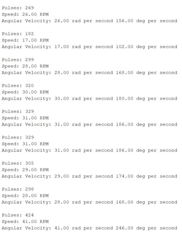
Open the Serial Monitor.
Here is the output when I rotate the motor forward:
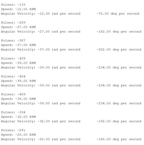
Here is the output when I rotate the motor in reverse.
Calculating Linear Velocity
Now that you know how to calculate the angular velocity of a wheel, you can calculate the linear velocity of that wheel if you know it’s radius. Here is the equation:
(Linear Velocity in meters per second) = (Radius of the wheel in meters) * (Angular Velocity in radians per second)


