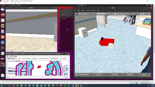
In this tutorial, I will show you have to perform auto-docking for a mobile robot using ROS 2, OpenCV, and an ArUco marker. Here is the output you will be able to generate if you follow this tutorial to the end:
Prerequisites
- ROS 2 Galactic installed on Ubuntu Linux 20.04
- You have already created a ROS 2 workspace. The name of my workspace is dev_ws.
- (Optional) You have completed this tutorial.
- (Optional) You have a package named two_wheeled_robot inside your ~/dev_ws/src folder, which I set up in this post. If you have another package, that is fine.
- (Optional) You have completed this tutorial on automatic docking.
- (Optional) You have completed this tutorial on how to perform pose estimation using an ArUco marker.
You can find the code for this post here on GitHub.
Version 1 – Harcode the ArUco Marker Pose
Create the Base Link to ArUco Marker Transform
Create a new transformation file between the base_link to aruco_marker.
cd ~/dev_ws/src/two_wheeled_robot/scripts/transforms/base_link_aruco_marker
gedit base_link_to_aruco_marker_transform.py
Add this code.
Save the file, and close it.
Change the execution permissions.
chmod +x base_link_to_aruco_marker_transform.py
Add the script to your CMakeLists.txt file.
Create a launch file.
cd ~/dev_ws/src/two_wheeled_robot/launch/hospital_world/
gedit hospital_world_connect_to_charging_dock_v5.launch.py
Add this code.
Save and close the file.
Create the Navigation to Charging Dock Script
Add a new navigate-to-charging-dock script. We will call it navigate_to_charging_dock_v3.py.
cd ~/dev_ws/src/two_wheeled_robot/scripts
gedit navigate_to_charging_dock_v3.py
Add this code.
Save the file, and close it.
Change the execution permissions.
chmod +x navigate_to_charging_dock_v3.py
Create Battery Status Publishers to Simulate the Robot’s Battery
Now let’s add a full battery publisher. This publisher indicates the battery has sufficient voltage for navigation in an environment.
gedit full_battery_pub.py
#!/usr/bin/env python3

"""
Description:
Publish the battery state at a specific time interval
In this case, the battery is a full battery.
-------
Publishing Topics:
/battery_status – sensor_msgs/BatteryState
-------
Subscription Topics:
None
-------
Author: Addison Sears-Collins
Website: AutomaticAddison.com
Date: January 13, 2022
"""

import rclpy # Import the ROS client library for Python
from rclpy.node import Node # Enables the use of rclpy's Node class
from sensor_msgs.msg import BatteryState # Enable use of the sensor_msgs/BatteryState message type

class BatteryStatePublisher(Node):
  """
  Create a BatteryStatePublisher class, which is a subclass of the Node class.
  The class publishes the battery state of an object at a specific time interval.
  """

  def __init__(self):
    """
    Class constructor to set up the node
    """

    # Initiate the Node class's constructor and give it a name
    super().__init__('battery_state_pub')

    # Create publisher(s)

    # This node publishes the state of the battery.
    # Maximum queue size of 10.
    self.publisher_battery_state = self.create_publisher(BatteryState, '/battery_status', 10)

    # Time interval in seconds
    timer_period = 0.1
    self.timer = self.create_timer(timer_period, self.get_battery_state)

    # Initialize battery level
    self.voltage = 9.0 # Initialize the battery voltage level
    self.percentage = 1.0  # Initialize the percentage charge level
    self.power_supply_status = 3 # Initialize the power supply status (e.g. NOT CHARGING)

  def get_battery_state(self):
    """
    Callback function.
    This function reports the battery state at the specific time interval.
    """
    msg = BatteryState() # Create a message of this type
    msg.voltage = self.voltage
    msg.percentage = self.percentage
    msg.power_supply_status = self.power_supply_status
    self.publisher_battery_state.publish(msg) # Publish BatteryState message

def main(args=None):

  # Initialize the rclpy library
  rclpy.init(args=args)

  # Create the node
  battery_state_pub = BatteryStatePublisher()

  # Spin the node so the callback function is called.
  # Publish any pending messages to the topics.
  rclpy.spin(battery_state_pub)

  # Destroy the node explicitly
  # (optional - otherwise it will be done automatically
  # when the garbage collector destroys the node object)
  battery_state_pub.destroy_node()

  # Shutdown the ROS client library for Python
  rclpy.shutdown()

if __name__ == '__main__':
  main()
Now let’s add a low battery publisher. This publisher indicates the battery is low.
cd ~/dev_ws/src/two_wheeled_robot/scripts/battery_state
gedit low_battery_pub.py
Now let’s add a charging battery publisher. This publisher indicates the battery is CHARGING (i.e. connected to the docking station).
cd ~/dev_ws/src/two_wheeled_robot/scripts/battery_state
gedit charging_battery_pub.py
Don’t forget to update CMakeLists.txt with these new scripts.
Launch the Robot
Open a new terminal window, and run the following node to indicate the battery is at full charge.
ros2 run two_wheeled_robot full_battery_pub.py
Open a new terminal and launch the robot.
ros2 launch two_wheeled_robot hospital_world_connect_to_charging_dock_v5.launch.py
Select the Nav2 Goal button at the top of RViz and click somewhere on the map to command the robot to navigate to any reachable goal location.
The robot will move to the goal location.
While the robot is moving, stop the full_battery_pub.py node.
CTRL + C
Now run this command to indicate low battery:
ros2 run two_wheeled_robot low_battery_pub.py
The robot will plan a path to the staging area and then move along that path.
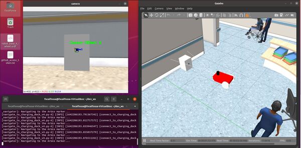
Once the robot reaches the staging area, the robot will navigate to the charging dock (i.e. ArUco marker) using the algorithm we developed earlier in this post. We assume the charging dock is located against a wall.
The algorithm (navigate_to_charging_dock_v3.py) works in four stages:
- Navigate to a staging area near the docking station once the battery gets below a certain level.
- Navigate to an imaginary line that is perpendicular to the face of the ArUco marker.
- Face the direction of the ArUco marker.
- Move straight towards the ArUco marker, making small heading adjustments along the way.
This script uses the static transform publisher for the ArUco marker. In other words, it assumes we have hardcoded the position and orientation of the ArUco marker ahead of time.
Once the robot has reached the charging dock, press CTRL + C to stop the low_battery_pub.py node, and type:
ros2 run two_wheeled_robot charging_battery_pub.py
That 1 for the power_supply_status indicates the battery is CHARGING.
Version 2: Do Not Hardcode the ArUco Marker Pose
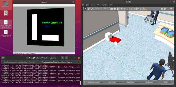
Let’s create another navigation-to-charging dock script. In this script, we assume we have not hardcoded the exact pose of the ArUco marker ahead of time. The algorithm (navigate_to_charging_dock_v4.py) works in four stages:
- Navigate to a staging area near the docking station once the battery gets below a certain level. This staging area is 1.5 meters in front of the docking station.
- Rotate around to search for the ArUco marker using the robot’s camera.
- Once the ArUco marker is detected, move towards it, making minor heading adjustments as necessary.
- Stop once the robot gets close enough (<0.22 meters from the LIDAR) to the charging dock (or starts charging).
- Undock once the robot gets to a full charge.
- Wait for the next navigation goal.
We assume the charging dock is located against a wall.
Create an ArUco Marker Centroid Offset Publisher and an ArUco Marker Detector Boolean Publisher
Let’s create a script that will detect an ArUco marker and publish the ArUco marker’s centroid offset (along the horizontal axis of the camera image).
Go into the scripts section of your package.
cd ~/dev_ws/src/two_wheeled_robot/scripts
gedit aruco_marker_detector.py
Add this code.
#!/usr/bin/env python3

# Detect an ArUco marker and publish the ArUco marker's centroid offset.
# The marker's centroid offset is along the horizontal axis of the camera image.
# Author:
# - Addison Sears-Collins
# - https://automaticaddison.com

# Import the necessary ROS 2 libraries
import rclpy # Python library for ROS 2
from rclpy.node import Node # Handles the creation of nodes
from rclpy.qos import qos_profile_sensor_data # Uses Best Effort reliability for camera
from cv_bridge import CvBridge # Package to convert between ROS and OpenCV Images
from geometry_msgs.msg import TransformStamped # Handles TransformStamped message
from sensor_msgs.msg import Image # Image is the message type
from std_msgs.msg import Bool # Handles boolean messages
from std_msgs.msg import Int32 # Handles int 32 type message

# Import Python libraries
import cv2 # OpenCV library
import numpy as np # Import Numpy library

# The different ArUco dictionaries built into the OpenCV library.
ARUCO_DICT = {
  "DICT_4X4_50": cv2.aruco.DICT_4X4_50,
  "DICT_4X4_100": cv2.aruco.DICT_4X4_100,
  "DICT_4X4_250": cv2.aruco.DICT_4X4_250,
  "DICT_4X4_1000": cv2.aruco.DICT_4X4_1000,
  "DICT_5X5_50": cv2.aruco.DICT_5X5_50,
  "DICT_5X5_100": cv2.aruco.DICT_5X5_100,
  "DICT_5X5_250": cv2.aruco.DICT_5X5_250,
  "DICT_5X5_1000": cv2.aruco.DICT_5X5_1000,
  "DICT_6X6_50": cv2.aruco.DICT_6X6_50,
  "DICT_6X6_100": cv2.aruco.DICT_6X6_100,
  "DICT_6X6_250": cv2.aruco.DICT_6X6_250,
  "DICT_6X6_1000": cv2.aruco.DICT_6X6_1000,
  "DICT_7X7_50": cv2.aruco.DICT_7X7_50,
  "DICT_7X7_100": cv2.aruco.DICT_7X7_100,
  "DICT_7X7_250": cv2.aruco.DICT_7X7_250,
  "DICT_7X7_1000": cv2.aruco.DICT_7X7_1000,
  "DICT_ARUCO_ORIGINAL": cv2.aruco.DICT_ARUCO_ORIGINAL
}

class ArucoNode(Node):
  """
  Create an ArucoNode class, which is a subclass of the Node class.
  """
  def __init__(self):
    """
    Class constructor to set up the node
    """
    # Initiate the Node class's constructor and give it a name
    super().__init__('aruco_node')

    # Declare parameters
    self.declare_parameter("aruco_dictionary_name", "DICT_ARUCO_ORIGINAL")
    self.declare_parameter("aruco_marker_side_length", 0.05)
    self.declare_parameter("camera_calibration_parameters_filename", "/home/focalfossa/dev_ws/src/two_wheeled_robot/scripts/calibration_chessboard.yaml")
    self.declare_parameter("image_topic", "/depth_camera/image_raw")
    self.declare_parameter("aruco_marker_name", "aruco_marker")

    # Read parameters
    aruco_dictionary_name = self.get_parameter("aruco_dictionary_name").get_parameter_value().string_value
    self.aruco_marker_side_length = self.get_parameter("aruco_marker_side_length").get_parameter_value().double_value
    self.camera_calibration_parameters_filename = self.get_parameter(
      "camera_calibration_parameters_filename").get_parameter_value().string_value
    image_topic = self.get_parameter("image_topic").get_parameter_value().string_value
    self.aruco_marker_name = self.get_parameter("aruco_marker_name").get_parameter_value().string_value

    # Check that we have a valid ArUco marker
    if ARUCO_DICT.get(aruco_dictionary_name, None) is None:
      self.get_logger().info("[INFO] ArUCo tag of '{}' is not supported".format(
        args["type"]))

    # Load the camera parameters from the saved file
    cv_file = cv2.FileStorage(
      self.camera_calibration_parameters_filename, cv2.FILE_STORAGE_READ)
    self.mtx = cv_file.getNode('K').mat()
    self.dst = cv_file.getNode('D').mat()
    cv_file.release()

    # Load the ArUco dictionary
    self.get_logger().info("[INFO] detecting '{}' markers...".format(
  	  aruco_dictionary_name))
    self.this_aruco_dictionary = cv2.aruco.Dictionary_get(ARUCO_DICT[aruco_dictionary_name])
    self.this_aruco_parameters = cv2.aruco.DetectorParameters_create()

    # Create the subscriber. This subscriber will receive an Image
    # from the image_topic.
    self.subscription = self.create_subscription(
      Image,
      image_topic,
      self.listener_callback,
      qos_profile=qos_profile_sensor_data)
    self.subscription # prevent unused variable warning

    # Create the publishers
    # Publishes if an ArUco marker was detected
    self.publisher_aruco_marker_detected = self.create_publisher(Bool, 'aruco_marker_detected', 10)

    # Publishes x-centroid offset with respect to the camera image
    self.publisher_offset_aruco_marker = self.create_publisher(Int32, 'aruco_marker_offset', 10)
    self.offset_aruco_marker = 0

    # Used to convert between ROS and OpenCV images
    self.bridge = CvBridge()

  def listener_callback(self, data):
    """
    Callback function.
    """
    # Convert ROS Image message to OpenCV image
    current_frame = self.bridge.imgmsg_to_cv2(data)

    # Detect ArUco markers in the video frame
    (corners, marker_ids, rejected) = cv2.aruco.detectMarkers(
      current_frame, self.this_aruco_dictionary, parameters=self.this_aruco_parameters,
      cameraMatrix=self.mtx, distCoeff=self.dst)

    # ArUco detected (True or False)
    aruco_detected_flag = Bool()
    aruco_detected_flag.data = False

    # ArUco center offset
    aruco_center_offset_msg = Int32()
    aruco_center_offset_msg.data = self.offset_aruco_marker

    image_width = current_frame.shape[1]

    # Check that at least one ArUco marker was detected
    if marker_ids is not None:

      # ArUco marker has been detected
      aruco_detected_flag.data = True

      # Draw a square around detected markers in the video frame
      cv2.aruco.drawDetectedMarkers(current_frame, corners, marker_ids)

      # Update the ArUco marker offset
      M = cv2.moments(corners[0][0])
      cX = int(M["m10"] / M["m00"])
      cY = int(M["m01"] / M["m00"])

      self.offset_aruco_marker = cX - int(image_width/2)
      aruco_center_offset_msg.data = self.offset_aruco_marker

      cv2.putText(current_frame, "Center Offset: " + str(self.offset_aruco_marker), (cX - 40, cY - 40),
        cv2.FONT_HERSHEY_COMPLEX, 0.7, (0, 255, 0), 2)

    # Publish if ArUco marker has been detected or not
    self.publisher_aruco_marker_detected.publish(aruco_detected_flag)

    # Publish the center offset of the ArUco marker
    self.publisher_offset_aruco_marker.publish(aruco_center_offset_msg)

    # Display image for testing
    cv2.imshow("camera", current_frame)
    cv2.waitKey(1)

def main(args=None):

  # Initialize the rclpy library
  rclpy.init(args=args)

  # Create the node
  aruco_node = ArucoNode()

  # Spin the node so the callback function is called.
  rclpy.spin(aruco_node)

  # Destroy the node explicitly
  # (optional - otherwise it will be done automatically
  # when the garbage collector destroys the node object)
  aruco_node.destroy_node()

  # Shutdown the ROS client library for Python
  rclpy.shutdown()

if __name__ == '__main__':
  main()
Save the script and close.
Add execution permissions.
chmod +x aruco_marker_detector.py
Add the file to your CMakeLists.txt.
Create the Navigation Script
Go into the scripts section of your package.
cd ~/dev_ws/src/two_wheeled_robot/scripts
gedit navigate_to_charging_dock_v4.py
Add this code.
Save the script and close.
Add execution permissions.
chmod +x navigate_to_charging_dock_v4.py
Add the file to your CMakeLists.txt.
Create the Launch File
cd ~/dev_ws/src/two_wheeled_robot/launch/hospital_world/
gedit hospital_world_connect_to_charging_dock_v6.launch.py
Add this code.
Save and close the file.
Launch the Robot
Open a new terminal window, and run the following node to indicate the battery is at full charge.
ros2 run two_wheeled_robot full_battery_pub.py
Open a new terminal and launch the robot.
ros2 launch two_wheeled_robot hospital_world_connect_to_charging_dock_v6.launch.py
Select the Nav2 Goal button at the top of RViz and click somewhere on the map to command the robot to navigate to any reachable goal location.
The robot will move to the goal location.
While the robot is moving, stop the full_battery_pub.py node.
CTRL + C
Now run this command to indicate low battery:
ros2 run two_wheeled_robot low_battery_pub.py
The robot will plan a path to the staging area and then move along that path.
Once the robot reaches the staging area, the robot will navigate to the charging dock (i.e. ArUco marker) using the algorithm we developed earlier in this post. We assume the charging dock is located against a wall.
Once the robot has reached the charging dock, press CTRL + C to stop the low_battery_pub.py node, and type:
ros2 run two_wheeled_robot charging_battery_pub.py
That 1 for the power_supply_status indicates the battery is CHARGING.
You can now simulate the robot reaching full charge by typing:
ros2 run two_wheeled_robot full_battery_pub.py
The robot will undock from the docking station.
You can then give the robot a new goal using the RViz Nav2 Goal button, and repeat the entire process again.
The Importance of Having a Rear Camera
In a humanoid robotic application, you can alter the algorithm so the robot backs into the charging dock. This assumes that you have a camera on the rear of the robot. You can see an implementation like this on this YouTube video.
The benefit of the robot backing into the charging dock is the robot is ready to navigate when it receives a goal….no backing up needed.
You can also add magnetic charging contacts like on this Youtube video to facilitate the connection.
That’s it! Keep building!