Partial Observability and Reinforcement Learning

In this post, I’m going to discuss how supervised learning can address the partial observability issue in reinforcement learning.

What is Partial Observability?

In a lot of the textbook examples of reinforcement learning, we assume that the agent, for example a robot, can perfectly observe the environment around it in order to extract relevant information about the current state. When this is the case, we say that the environment around the agent is fully observable

However, in many cases, such as in the real world, the environment is not always fully observable. For example, there might be noisy sensors, missing information about the state, or outside interferences that prohibit an agent from being able to develop an accurate picture of the state of its surrounding environment. When this is the case, we say that the environment is partially observable.

Let us take a look at an example of partial observability using the classic cart-pole balancing task that is often found in discussions on reinforcement learning.

Below is a video demonstrating the cart-pole balancing task. The goal is to keep to keep a pole from falling over by making small adjustments to the cart support underneath the pole.

In the video above, the agent learns to keep the pole balanced for 30 minutes after 600 trials. The state of the world consists of two parts:

  1. The pole angle
  2. The angular velocity

However, what happens if one of those parts is missing? For example, the pole angle reading might disappear. 

Also, what happens if the readings are noisy, where the pole angle and angular velocity measurements deviate significantly from the true value? 

In these cases, a reinforcement learning policy that depends only on the current observation xt (where x is the pole angle or angular velocity value and time t) will suffer in performance. This in a nutshell is the partial observability problem that is inherent in reinforcement learning techniques.

Addressing Partial Observability Using Long Short-Term Memory (LSTM) Networks

One strategy for addressing the partial observability problem (where information about the actual state of the environment is missing or noisy) is to use long short-term memory neural networks. In contrast to artificial feedforward neural networks which have a one-way flow of information from the input layer, LSTMs have feedback connections. Past information persists from run to run of the network, giving the system a “memory.” This memory can then be used to make predictions about the current state of the environment.

The details of exactly how the memory explained above is created is described in this paper written by Bram Baker of the Unit of Experimental and Theoretical Psychology at Leyden University. Baker showed that LSTM neural networks can help improve reinforcement learning policies by creating a “belief state.” This “belief state” is based on probabilities of reward, state transitions, and observations, given prior states and actions. 

Thus, when the actual state (as measured by a robot’s sensor for example) is unavailable or super noisy, an agent can use belief state information generated by an LSTM to determine the appropriate action to take.

Combining Deep Neural Networks With Reinforcement Learning for Improved Performance

The performance of reinforcement learning can be improved by incorporating supervised learning techniques. Let us take a look at a concrete example.

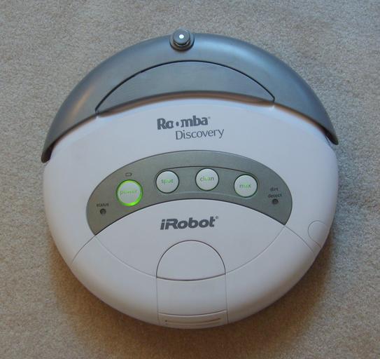
You all might be familiar with the Roomba robot created by iRobot. The Roomba robot is perhaps the most popular robot vacuum sold in the United States. 

roomba_discovery

The Roomba is completely autonomous, moving around the room with ease, cleaning up dust, pet hair, and dirt along the way. In order to do its job, the Roomba contains a number of sensors that enable it to perceive the current state of the environment (i.e. your house). 

Let us suppose that the Roomba is governed by a reinforcement learning policy. This learning policy could be improved if we have accurate readings of the current state of the environment. And one way to improve these readings is to incorporate computer vision.

Since reinforcement learning depends heavily on accurate readings of the current state of the environment, we could use deep neural networks (a supervised learning technique) to pre-train the robot so that it can perform common computer vision tasks such as recognizing objects, localizing objects, and classifying objects before we even start running the reinforcement learning algorithm. These “readings” would improve the state portion of the reinforcement learning loop.

Deep neural networks have already displayed remarkable accuracy for computer vision problems. We can use these techniques to enable the robot to get a more accurate reading of the current state of the environment so that it can then take the most appropriate actions towards maximizing cumulative reward.

Boltzmann Distribution and Epsilon Greedy Search

How Does the Boltzmann Distribution Fit Into the Discussion of Epsilon Greedy Search?

In order to answer your question, let us take a closer look at the definition of epsilon greedy search. With our knowledge of how that works, we can then see how the Boltzmann distribution fits into the discussion of epsilon greedy search.

What is Epsilon Greedy Search?

When you are training an agent (e.g. race car, robot, etc.) with an algorithm like Q-learning, you can either have the agent take a random action with probability ϵ or have the agent be greedy and take the action that corresponds to its policy with probability 1-ϵ (i.e. the action for a given state that has the highest Q-value). The former is known as exploration while the latter is called exploitation. In reinforcement learning, we have this constant dichotomy of:

  • exploration vs. exploitation
  • learn vs. earn
  • not greedy vs. greedy
  • Exploration: Try a new bar in your city.
  • Exploitation: Go to the same watering hole you have been going to for decades.
  • Exploration: Start a business.
  • Exploitation: Get a job.
  • Exploration: Try to make new friends.
  • Exploitation: Keep inviting over your college buddies.
  • Exploration: Download Tinder dating app.
  • Exploitation: Call the ex.
  • Exploration (with probability ϵ): Gather more information about the environment.
  • Exploitation (with probability 1-ϵ): Make a decision based on the best information (i.e. policy) that is currently available.

The epsilon greedy algorithm in which ϵ is 0.20 says that most of the time the agent will select the trusted action a, the one prescribed by its policy π(s) -> a. However, 20% of the time, the agent will choose a random action instead of following its policy. 

We often want to have the epsilon-greedy algorithm in place for a reinforcement learning problem because often what is best for the agent long term (e.g. trying something totally random that pays off in a big way down the road) might not be the best for the agent in the short term (e.g. sticking with the best option we already know).

What Does the Boltzmann Distribution Have to Do With Epsilon Greedy Search?

Notice in the epsilon greedy search section above, I said that 20% of the time the agent will choose a random action instead of following its policy. The problem with this is that it treats all actions equally when making a decision on what action to take. What happens though if some actions might look more promising than others? Plain old epsilon greedy search cannot handle a situation like this. The fact is that, in the real world, all actions are not created equal.

A common method is to use the Boltzmann distribution (also known as Gibbs distribution). Rather than blindly accepting any random action when it comes time for the agent to explore the environment from a given state s, the agent selections an action a (from a set of actions A) with probability:

boltzmann-distribution

What this system is doing above is ranking and weighting all actions in the set of possible actions based on their Q-values. This system is often referred to as softmax selection rules.

Take a closer look at the equation above to see what we are doing here. A really high value of tau means that all actions are equally likely to be selected because we are diluting the impact of the Q-values for each action (by dividing by tau). However, as tau gets lower and lower, there will be greater differences in the selection probabilities for each action. The action with the highest Q[s,a] value is therefore much more likely to get selected. And when tau gets close to zero, the Boltzmann selection criteria I outlined above becomes indistinguishable from greedy search. For an extremely low value of tau, the agent will select the action with the highest Q-value and therefore never explore the environment via a random action.