In this tutorial, we will learn how to create a service and a client in ROS 2 Foxy Fitzroy using Python. The client-service relationship in ROS 2 is a request-reply relationship. A client node sends a request for data to the service node. The service node then sends a reply to the client node.
A real-world example of this is a client node requesting sensor data from a service node. The service node then responds to the client node with the requested sensor data.
A file called a .srv file defines the structure of the service-client node interaction.

The example we will use here is an addition system. We will create a client node that requests the sum of two integers. We will then create a service node that will respond to the client node with the sum of those two integers.
The official tutorial is located in the ROS 2 Foxy documentation, but we’ll run through the entire process step-by-step below.
You Will Need
In order to complete this tutorial, you will need:
Prerequisites
You have already created a workspace.
Create a Package
Open a new terminal window, and navigate to the src directory of your workspace:
cd ~/dev_ws/src
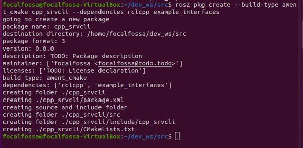
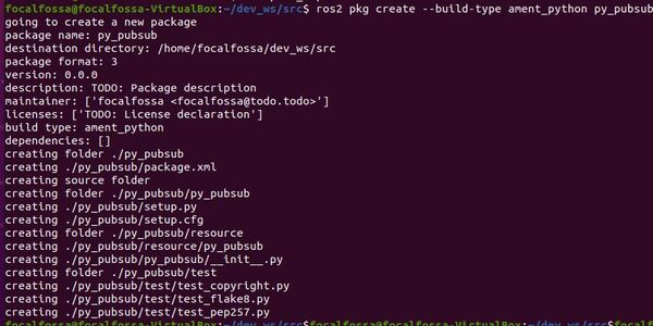
Now let’s create a package named py_srvcli.
Type this command:
ros2 pkg create --build-type ament_python py_srvcli --dependencies rclpy example_interfaces
Your package named py_srvcli has now been created.
You will note that we added the –dependencies command after the package creation command. Doing this automatically adds the dependencies to your package.xml file.
Modify Package.xml
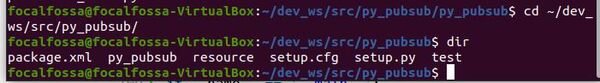
Go to the dev_ws/src/py_srvcli folder.
cd ~/dev_ws/src/py_srvcli
Make sure you have a text editor installed. I like to use gedit.
sudo apt-get install gedit
Open the package.xml file.
gedit package.xml
Fill in the description of the py_srvcli package, your email address and name on the maintainer line, and the license you desire (e.g. Apache License 2.0).
<description>A minimal Python client and service node</description>
<maintainer email="automaticaddison@todo.todo">automaticaddison</maintainer>
<license>Apache License 2.0</license>
Save and close the file.
Write a Service Node
Move to the dev_ws/src/py_srvcli/py_srvcli folder.
cd ~/dev_ws/src/py_srvcli/py_srvcli
Create a new Python file named add_two_ints_server.py
gedit add_two_ints_server.py
Write the following code. Don’t be intimidated. Just go one line at a time and read the comments to understand what each line does.
This service node adds two integers together.
# Import AddTwoInts service type from the example_interfaces package
from example_interfaces.srv import AddTwoInts

# ROS 2 Client Library for Python
import rclpy

# Handles nodes
from rclpy.node import Node

class MinimalService(Node):

    def __init__(self):
        # Initialize the node via this constructor
        super().__init__('minimal_service')

        # Create a service
        self.srv = self.create_service(AddTwoInts, 'add_two_ints', self.add_two_ints_callback)

    def add_two_ints_callback(self, request, response):
        # Receive the request data and sum it
        response.sum = request.a + request.b

        # Return the sum as the reply
        self.get_logger().info('Incoming request\na: %d b: %d' % (request.a, request.b))
        return response

def main(args=None):

    # Start ROS
    rclpy.init(args=args)

    # Create the service
    minimal_service = MinimalService()

    # Make the service available to the network
    rclpy.spin(minimal_service)

    # Shutdown ROS
    rclpy.shutdown()

if __name__ == '__main__':
    main()
Save the file, and close it.
Modify Setup.py
Go to the following directory.
cd ~/dev_ws/src/py_srvcli/
Open setup.py.
gedit setup.py
Add the following line between the ‘console_scripts’: brackets:
'service = py_srvcli.add_two_ints_server:main',
Save the file, and close it.
Write a Client Node
Move to the dev_ws/src/py_srvcli/py_srvcli folder.
cd ~/dev_ws/src/py_srvcli/py_srvcli
Create a new Python file named add_two_ints_client.py
gedit add_two_ints_client.py
Write the following code. Don’t be intimidated. Just go one line at a time and read the comments to understand what each line does.
# Enables command line input
import sys

from example_interfaces.srv import AddTwoInts
import rclpy
from rclpy.node import Node

class MinimalClientAsync(Node):

    def __init__(self):
        # Create a client
        super().__init__('minimal_client_async')
        self.cli = self.create_client(AddTwoInts, 'add_two_ints')

        # Check if the a service is available
        while not self.cli.wait_for_service(timeout_sec=1.0):
            self.get_logger().info('service not available, waiting again...')
        self.req = AddTwoInts.Request()

    def send_request(self):
        self.req.a = int(sys.argv[1])
        self.req.b = int(sys.argv[2])
        self.future = self.cli.call_async(self.req)


def main(args=None):
    rclpy.init(args=args)

    minimal_client = MinimalClientAsync()
    minimal_client.send_request()

    while rclpy.ok():
        rclpy.spin_once(minimal_client)
        # See if the service has replied
        if minimal_client.future.done():
            try:
                response = minimal_client.future.result()
            except Exception as e:
                minimal_client.get_logger().info(
                    'Service call failed %r' % (e,))
            else:
                minimal_client.get_logger().info(
                    'Result of add_two_ints: for %d + %d = %d' %
                    (minimal_client.req.a, minimal_client.req.b, response.sum))
            break

    minimal_client.destroy_node()
    rclpy.shutdown()


if __name__ == '__main__':
    main()
Save the file, and close it.
Modify Setup.py
Go to the following directory.
cd ~/dev_ws/src/py_srvcli/
Open setup.py.
gedit setup.py
Make sure the entry_points block looks like this:
entry_points={
    'console_scripts': [
        'service = py_srvcli.add_two_ints_server:main',
        'client = py_srvcli.add_two_ints_client:main',
    ],
},
Save the file, and close it.
Build the Package
Return to the root of your workspace:
cd ~/dev_ws/
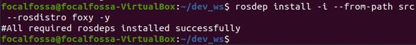
We need to double check that all the dependencies needed are already installed.
rosdep install -i --from-path src --rosdistro foxy -y
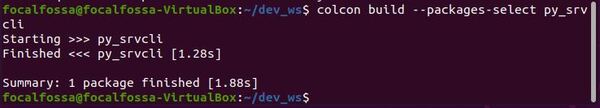
Build the package:
colcon build --packages-select py_srvcli
Run the Nodes
To run the nodes, open a new terminal window.
Make sure you are in the root of your workspace:
cd ~/dev_ws/
Run the service node.
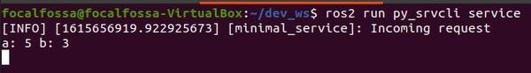
ros2 run py_srvcli service
Open a new terminal, and run the client node. At the end of the command, put the two integers you would like to add.
ros2 run py_srvcli client 5 3
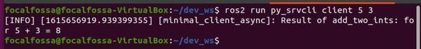
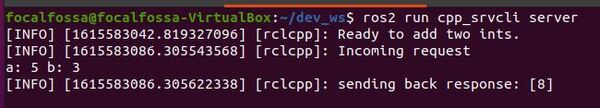
Go back to the service node terminal. Here is what I see:
When you’re done, press CTRL + C in all terminal windows to shut everything down.
That’s it. Keep building!