In this tutorial, we will write a basic C++ program for NVIDIA Jetson Nano.
Prerequisites
- You have already set up your NVIDIA Jetson Nano.
- This tutorial will be similar to my C++ fundamentals for robotics tutorial.
Check Your GCC Version
Open a terminal window, and run the following command to see the version of the GCC C/C++ compiler you have.
gcc --version
If gcc is not installed, follow the instructions in the next section.
Install the GCC/G++ Compilers
Open a new terminal window, and type:
sudo apt-get update
Now use this command to install a bunch of packages, including GCC, G++, and GNU Make:
sudo apt install build-essential
You might see some sort of error about things being locked if you try the following command. If you do, kill all processes that are using the APT package management tool using this command:
sudo killall apt apt-get
Remove the lock files:
sudo rm /var/lib/apt/lists/lock
sudo rm /var/cache/apt/archives/lock
sudo rm /var/lib/dpkg/lock*
Reconfigure the packages and update:
sudo dpkg --configure -a
sudo apt update
Now use this command to install numerous packages, including GCC, G++, and GNU Make:
sudo apt install build-essential
Press Y to continue.
Wait while the whole thing downloads.
Now, install the manual pages about using GNU/Linux for development (note: it might already be installed):
sudo apt-get install manpages-dev
Check to see if both GCC and G++ are installed.
whereis gcc
whereis g++
Check what version you have.
gcc --version
g++ --version
Install the C/C++ Debugger
In this section, we will install the C/C++ debugger. It is called GNU Debugger (GDB) and enables us to detect problems or bugs in the code that we write.
In the terminal window, type the following command:
sudo apt-get install gdb
You will be asked to type your password, and then click Enter.
Type the following command to verify that it is installed:
gdb
Type this command to quit.
quit
Press Enter.
Exit the terminal.
exit
Install Gedit
Install gedit, a text editor that will enable us to write code in C/C++.
Open a terminal window, and type:
sudo apt-get install gedit
Write a Hello World Program in C
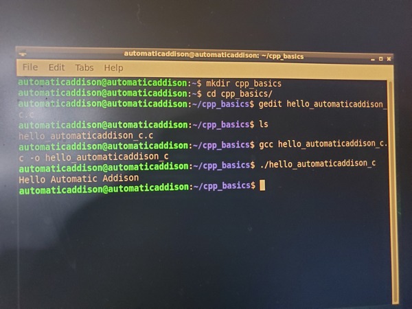
Let’s write a program that does nothing but print “Hello Automatic Addison” (i.e. my version of a “Hello World” program) to the screen.
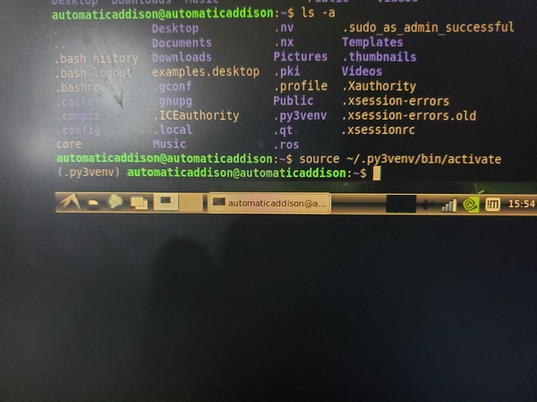
Open a new terminal window, and create a new folder.
mkdir cpp_basics
Move to that folder.
cd cpp_basics
Open a new C program.
gedit hello_automaticaddison_c.c
#include<stdio.h>
int main()
{
printf("Hello Automatic Addison\n");
return 0;
}
Save the file, and close it.
See if your file is in there.
ls
Compile the program.
gcc hello_automaticaddison_c.c -o hello_automaticaddison_c
Run the program.
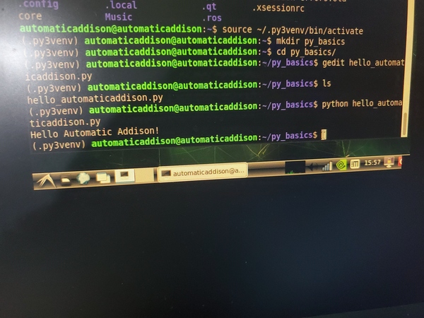
./hello_automaticaddison_c
Here is what I see.
Write a Hello World Program in C++
Open a new C++ program.
gedit hello_automaticaddison_cpp.cpp
Write the following code.
// Simple C++ program to display "Hello Automatic Addison"

// Header file for input output functions
#include<iostream>

using namespace std;

// main function
// where the execution of program begins
int main()
{
    // prints hello world
    cout<<"Hello Automatic Addison";

    return 0;
}
Save the file, and close it.
See if your file is in there.
ls
Compile the program. All of this is just a single command.
g++ -o hello_automaticaddison_cpp hello_automaticaddison_cpp.cpp
If you see an error, check your program to see if it is exactly like I wrote it.
Run the program.
./hello_automaticaddison_cpp
Here is what I see.
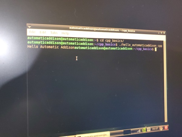
That’s it. Keep building!