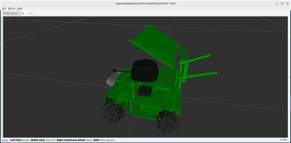
In this tutorial, we will create a model of a mobile robot from scratch. Our robot model will be in the standard Unified Robot Description Format (URDF).
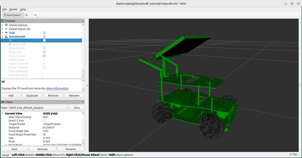
By the end of this tutorial, you will be able to build this:

We will then visualize the robot in RViz, a 3D visualization tool for ROS 2.
The official tutorial for creating a URDF file is here on the ROS 2 website; but that tutorial only deals with a fictitious robot.
It is far more fun and helpful to show you how to create a URDF file for a real-world robot, like the ones you will work with at your job or at school…like this one, for example…the Kuka omniMove robot used in an Airbus facility in Germany to move aircraft parts around the factory floor:
You can see this Kuka robot has mecanum wheels. The robot we will build in this tutorial will have mecanum wheels, also known as an omnidirectional robot. A mecanum wheel robot uses special wheels with rollers attached at an angle, allowing it to move in any direction by rotating the wheels independently.
Compared to robots with standard wheels that can only move forward, backward, and turn, mecanum wheel robots have greater maneuverability and can move sideways without changing orientation.
Within ROS 2, defining the URDF file of your mobile robot is important because it allows software tools to understand the robot’s structure, enabling tasks like simulation, motion planning, and sensor data interpretation. It is like giving the robot a digital body that software can interact with.
I will walk through all the steps below for creating the URDF for the ROSMASTER X3 by Yahboom, a company that makes educational robots.
Follow along with me click by click, keystroke by keystroke.
If you prefer to learn by video instead of text, you can follow the complete tutorial here:
Prerequisites
- You have completed this tutorial: Create and Visualize a Robotic Arm with URDF – ROS 2 Jazzy (recommended)
- I am assuming you are using Visual Studio Code, but you can use any code editor.
You can find all the code here on GitHub.
References
- Yahboom Website (Makers of the robot we will model in this video)
- Yahboom GitHub
- ROSMASTER X3 Study Guide by Yahboom
Here is my GitHub repository for this project.
Create a Package
The first step is to create a ROS 2 package to store all your files.
Open a new terminal window, and create a new folder named yahboom_rosmaster.
cd ~/ros2_ws/srcmkdir yahboom_rosmastercd yahboom_rosmasterNow create the package where we will store our URDF file.
ros2 pkg create --build-type ament_cmake --license BSD-3-Clause yahboom_rosmaster_descriptionNow, let’s create a metapackage.
I discuss the purpose of a metapackage in this post.
A metapackage doesn’t contain anything except a list of dependencies to other packages. You can use a metapackage to make it easier to install multiple related packages at once.
If you were to make your package available to install publicly using the apt-get package manager on Ubuntu for example, a metapackage would enable someone to automatically install all the ROS2 packages that are referenced in your metapackage.
ros2 pkg create --build-type ament_cmake --license BSD-3-Clause yahboom_rosmastercd yahboom_rosmasterConfigure your package.xml file.
gedit package.xmlMake your package.xml file look like this:
<?xml version="1.0"?>
<?xml-model href="http://download.ros.org/schema/package_format3.xsd" schematypens="http://www.w3.org/2001/XMLSchema"?>
<package format="3">
  <name>yahboom_rosmaster</name>
  <version>0.0.0</version>
  <description>ROSMASTER series robots by Yahboom (metapackage).</description>
  <maintainer email="automaticaddison@todo.todo">ubuntu</maintainer>
  <license>BSD-3-Clause</license>

  <buildtool_depend>ament_cmake</buildtool_depend>

  <exec_depend>yahboom_rosmaster_description</exec_depend>

  <test_depend>ament_lint_auto</test_depend>
  <test_depend>ament_lint_common</test_depend>

  <export>
    <build_type>ament_cmake</build_type>
  </export>
</package>
Add a README.md to describe what the package is about.
cd ..gedit README.md
# yahboom_rosmaster #


I also recommend adding placeholder README.md files to the yahboom_rosmaster folder.
# yahboom_rosmaster #
The yahboom_rosmaster package is a metapackage. It contains lists of dependencies to other packages.
… as well as the yahboom_rosmaster_description folder.
# yahboom_rosmaster_description #
The yahboom_rosmaster_description package contains the robot description files that define the physical aspects of a robot, including its geometry, kinematics, dynamics, and visual aspects.
Now let’s build our new package:
cd ~/ros2_wscolcon buildLet’s see if our new package is recognized by ROS 2.
Either open a new terminal window or source the bashrc file like this:
source ~/.bashrc
ros2 pkg listYou can see the newly created packages right there at the bottom.

Now let’s create the following folders:
mkdir -p ~/ros2_ws/src/yahboom_rosmaster/yahboom_rosmaster_description/meshes/rosmaster_x3/visual
mkdir -p ~/ros2_ws/src/yahboom_rosmaster/yahboom_rosmaster_description/urdf/control
mkdir -p ~/ros2_ws/src/yahboom_rosmaster/yahboom_rosmaster_description/urdf/mech
mkdir -p ~/ros2_ws/src/yahboom_rosmaster/yahboom_rosmaster_description/urdf/sensors
mkdir -p ~/ros2_ws/src/yahboom_rosmaster/yahboom_rosmaster_description/urdf/robots/
Add the Meshes
Mesh files are what make your robot look realistic in robotics simulation and visualization programs.
Mesh files visually represent the 3D shape of the robot parts. These files are typically in formats such as STL (Stereo Lithography – .stl) or COLLADA (.dae).
The mesh files we are going to use were already available in the GitHub repository managed by Yahboom. We didn’t have to create these files from scratch. I got them from the manufacturer’s website.
However, if you want to create your own custom 3D printed mobile robot in the future, for example, you can make your own mesh file. Here is how:
- Design the robot’s body using CAD programs like Onshape, Fusion 360, AutoCAD, or Solidworks. These tools help you create 3D models of the robot parts.
- Export the 3D models as mesh files in formats like STL or COLLADA. These files contain information about the robot’s shape, including vertices, edges, and faces.
- If needed, use a tool like Blender to simplify the mesh files. This makes them easier to use in simulations and visualizations.
- Add the simplified mesh files to your URDF file to visually represent what the robot looks like.
Let’s pull these mesh files off GitHub.
First, open a new terminal window, and type:
cd ~/Downloads/Clone the yahboom_rosmaster repository to your machine.
git clone https://github.com/automaticaddison/yahboom_rosmaster.gitMove to the mesh files for the robot we are going to model:
cp -r yahboom_rosmaster/yahboom_rosmaster_description/meshes/* ~/ros2_ws/src/yahboom_rosmaster/yahboom_rosmaster_description/meshes/ls ~/ros2_ws/src/yahboom_rosmaster/yahboom_rosmaster_description/meshes/rosmaster_x3/visual/You can see the mesh files (.stl) for the robot.
Configure CMakeLists.txt
Let’s open Visual Studio Code.
cd ~/ros2_ws/src/yahboom_rosmaster/code .Configure the CMakeLists.txt for the yahboom_rosmaster_description package. Make sure it looks like this:
cmake_minimum_required(VERSION 3.8)
project(yahboom_rosmaster_description)

# Check if the compiler being used is GNU's C++ compiler (g++) or Clang.
# Add compiler flags for all targets that will be defined later in the
# CMakeLists file. These flags enable extra warnings to help catch
# potential issues in the code.
# Add options to the compilation process
if(CMAKE_COMPILER_IS_GNUCXX OR CMAKE_CXX_COMPILER_ID MATCHES "Clang")
  add_compile_options(-Wall -Wextra -Wpedantic)
endif()

# Locate and configure packages required by the project.
find_package(ament_cmake REQUIRED)
find_package(urdf_tutorial REQUIRED)

# Copy necessary files to designated locations in the project
install (
  DIRECTORY meshes urdf
  DESTINATION share/${PROJECT_NAME}
)

# Automates the process of setting up linting for the package, which
# is the process of running tools that analyze the code for potential
# errors, style issues, and other discrepancies that do not adhere to
# specified coding standards or best practices.
if(BUILD_TESTING)
  find_package(ament_lint_auto REQUIRED)
  # the following line skips the linter which checks for copyrights
  # comment the line when a copyright and license is added to all source files
  set(ament_cmake_copyright_FOUND TRUE)
  # the following line skips cpplint (only works in a git repo)
  # comment the line when this package is in a git repo and when
  # a copyright and license is added to all source files
  set(ament_cmake_cpplint_FOUND TRUE)
  ament_lint_auto_find_test_dependencies()
endif()

ament_package()
Configure package.xml
Make sure your package.xml for the yahboom_rosmaster_description package looks like this:
<?xml version="1.0"?>
<?xml-model href="http://download.ros.org/schema/package_format3.xsd" schematypens="http://www.w3.org/2001/XMLSchema"?>
<package format="3">
  <name>yahboom_rosmaster_description</name>
  <version>0.0.0</version>
  <description>Contains the robot description files that define the physical
    aspects of a robot, including its geometry, kinematics, dynamics, and
    visual aspects.</description>
  <maintainer email="automaticaddison@todo.todo">ubuntu</maintainer>
  <license>BSD-3-Clause</license>

  <buildtool_depend>ament_cmake</buildtool_depend>
  <depend>urdf_tutorial</depend>

  <test_depend>ament_lint_auto</test_depend>
  <test_depend>ament_lint_common</test_depend>

  <export>
    <build_type>ament_cmake</build_type>
  </export>
</package>
Build the Package
Now let’s build the package.
cd ~/ros2_ws/rosdep install -i --from-path src --rosdistro $ROS_DISTRO -yYou should see:
#All required rosdeps installed successfullyIf not, type your password, and install the required dependencies.
Open a terminal window, and type:
buildIf this command doesn’t work, type these commands:
echo "alias build='cd ~/ros2_ws/ && colcon build && source ~/.bashrc'" >> ~/.bashrcbuildCreate the URDF File
Now let’s create our URDF file. We will actually create it in XACRO format. I will use the terms URDF and XACRO interchangeably going forward.
XACRO files are like blueprints for URDF files, using macros and variables to simplify complex robot descriptions.
Imagine XACRO as the architect drawing up plans, and URDF as the final, ready-to-use construction document. Both file types represent the robotic arm, but XACRO offers more flexibility and organization.
Before a ROS tool or component can use the information in a XACRO file, it must first be processed (translated) into a URDF file. This step allows for the dynamic generation of robot descriptions based on the specific configurations defined in the XACRO file.
Open a terminal window, and type this command to create all the files we need:
touch ~/ros2_ws/src/yahboom_rosmaster/yahboom_rosmaster_description/urdf/mech/{rosmaster_x3_base.urdf.xacro,mecanum_wheel.urdf.xacro} ~/ros2_ws/src/yahboom_rosmaster/yahboom_rosmaster_description/urdf/sensors/{rgbd_camera.urdf.xacro,imu.urdf.xacro,lidar.urdf.xacro} ~/ros2_ws/src/yahboom_rosmaster/yahboom_rosmaster_description/urdf/robots/rosmaster_x3.urdf.xacro
Robot Base
Let’s start with creating our base: rosmaster_x3_base.urdf.xacro. Add this code.
Robot Wheels
Now let’s create a generic mecanum wheel: mecanum_wheel.urdf.xacro. Add this code.
RGBD Camera
Now let’s create the RGBD camera: rgbd_camera.urdf.xacro. An RGBD camera is like a regular digital camera that not only captures colors (RGB) but also measures how far away everything in the scene is from the camera (the D stands for depth). This added depth information allows the camera to create 3D maps of its surroundings.
You can find a big repository of sensors that can be implemented in simulation for Gazebo in this GitHub repository.
Add this code.
Robot LIDAR
Now let’s create the LIDAR: lidar.urdf.xacro. We will add the LIDAR plugin so we can generate simulated LIDAR data in a future tutorial.
Add this code.
Robot Inertial Measurement Unit (IMU)
Now let’s create the IMU: imu.urdf.xacro. An IMU (Inertial Measurement Unit) is a sensor that measures movement, specifically acceleration, rotation, and sometimes magnetic fields, to help determine an object’s position and motion.
Add this code.
Full Robot
Now let’s create the full robot, bringing together all the components we have created: rosmaster_x3.urdf.xacro. Add this code.
Understanding the URDF
Let’s walk through each file so we can understand what is going on.
rosmaster_x3_base.urdf.xacro
At the top, we start with an XML declaration and define that this is a robot description using xacro, which is like a macro language for robot descriptions:
<?xml version="1.0"?>
<robot xmlns:xacro="http://www.ros.org/wiki/xacro">
Then we have a bunch of properties that define the robot’s dimensions in meters:
<xacro:property name="total_width" value="0.19940" />  <!-- About 20cm wide -->
<xacro:property name="wheel_width" value="0.0304" />   <!-- About 3cm wheel width -->
<xacro:property name="wheel_radius" value="0.0325" />  <!-- About 3.25cm wheel radius -->
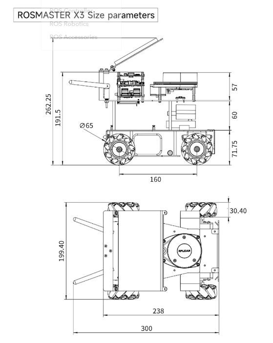
The code defines a macro called “rosmaster_x3_base” – think of this like a template for the robot’s base. The base has several important parts.
The base_link is the main body of the robot. It has three important sections:
- visual: This defines how the robot looks in simulation using a 3D model file (STL)
- collision: This is a simplified box shape used to detect when the robot hits things
- inertial: This defines the robot’s mass and how its weight is distributed
<link name="${prefix}base_link">
    <visual>
        <!-- The robot's appearance -->
        <geometry>
            <mesh filename="file://$(find yahboom_rosmaster_description)/meshes/rosmaster_x3/visual/base_link_X3.STL"/>
        </geometry>
        <!-- Makes it green -->
        <material name="green">
          <color rgba="0 0.7 0 1"/>
        </material>
    </visual>
    <!-- Other parts... -->
</link>
The gazebo tag adds special properties for the Gazebo simulator, like how the material looks in different lighting:
<gazebo reference="${prefix}base_link">
    <visual>
        <material>
            <ambient>0 0.7 0 1</ambient>
            <diffuse>0 0.7 0 1</diffuse>
            <specular>0 0.7 0 1</specular>
        </material>
    </visual>
</gazebo>
The math in the inertial section (ixx, iyy, izz) describes how the robot resists rotation around different axes – this is important for realistic physics simulation. The formula used is the standard equation for the moment of inertia of a rectangular box.
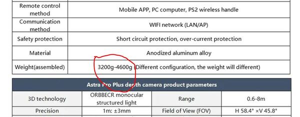
mecanum_wheel.urdf.xacro
Unlike regular wheels that can only move forward and backward, mecanum wheels have small rollers arranged at 45-degree angles around their circumference. This unique design allows a robot to move sideways, diagonally, or even rotate in place while remaining stationary – similar to how a crab can walk sideways.
In this file, we start with the basic properties of our wheel. These measurements define the physical characteristics:
<xacro:property name="wheel_radius" value="0.0325" />      <!-- Wheel is 6.5cm in diameter -->
<xacro:property name="wheel_separation" value="0.169" />   <!-- Distance between left and right wheels -->
<xacro:property name="wheel_width" value="0.03040" />     <!-- How thick the wheel is -->
<xacro:property name="wheel_mass" value="0.1" />          <!-- Wheel weighs 0.1 kg -->
<xacro:property name="wheel_xoff" value="0.08" />         <!-- How far forward/back the wheel is -->
<xacro:property name="wheel_yoff" value="-0.01" />        <!-- Small sideways offset -->
The wheel radius affects how fast the robot moves for a given motor speed.
The separation between wheels influences turning behavior – wider-set wheels provide more stability but require more torque to turn.
The mass and dimensions affect the robot’s physics simulation, including momentum and inertia.
Next, we define a macro – think of it as a template – that we can use to create wheels:
<xacro:macro name="mecanum_wheel" params="prefix side x_reflect y_reflect">
This macro is clever – instead of writing separate code for each wheel, we write it once and use parameters to customize it. The prefix parameter helps us name each wheel uniquely (like “front_left_wheel” or “rear_right_wheel”). The x_reflect and y_reflect parameters are either 1 or -1, letting us mirror the wheel’s position and orientation for different corners of the robot.
The visual component defines what we see in the simulator:
<visual>
    <origin xyz="0 0 0" rpy="${pi/2} 0 0"/>   <!-- Rotated 90 degrees around X axis -->
    <geometry>
        <mesh filename="file://$(find yahboom_rosmaster_description)/meshes/rosmaster_x3/visual/${side}_wheel_X3.STL"/>
    </geometry>
    <material name="dark_gray">
        <color rgba="0.2 0.2 0.2 1.0"/>       <!-- Dark gray color -->
    </material>
</visual>
This section loads a 3D model (STL file) of the wheel. The rotation parameters (rpy = roll, pitch, yaw) ensure the wheel is oriented correctly. The dark gray color makes it easy to distinguish from other robot parts.
For physics simulation, we need a collision model. While the visual model can be complex and detailed, the collision model is kept simple for computational efficiency:
<collision>
    <geometry>
        <cylinder radius="${wheel_radius}" length="${wheel_width}"/>
    </geometry>
</collision>
Instead of using the detailed STL model for collision detection, we use a simple cylinder. This significantly speeds up physics calculations while maintaining reasonable accuracy.
The inertial properties define how the wheel behaves physically:
<inertial>
    <mass value="${wheel_mass}"/>
    <inertia
        ixx="${(wheel_mass/12.0) * (3*wheel_radius*wheel_radius + wheel_width*wheel_width)}"
        iyy="${(wheel_mass/2.0) * (wheel_radius*wheel_radius)}"
        izz="${(wheel_mass/12.0) * (3*wheel_radius*wheel_radius + wheel_width*wheel_width)}"/>
</inertial>
These seemingly complex formulas are based on physics equations for a cylinder’s moment of inertia. They determine how the wheel resists changes in rotation around different axes.
The joint configuration defines how the wheel connects to the robot:
<joint name="${prefix}${side}_wheel_joint" type="continuous">
    <axis xyz="0 1 0"/>                <!-- Spins around Y axis -->
    <parent link="${prefix}base_link"/>
    <child link="${prefix}${side}_wheel_link"/>
    <!-- Position is calculated based on x_reflect and y_reflect to place wheel correctly -->
    <origin xyz="${x_reflect*wheel_xoff} ${y_reflect*(wheel_separation/2+wheel_yoff)} ${-wheel_radius}" rpy="0 0 0"/>
</joint>
A “continuous” joint means it can rotate indefinitely in either direction. The axis specification (0 1 0) means it rotates around the Y axis of the parent link.
The origin calculation uses our x_reflect and y_reflect parameters to position each wheel correctly relative to the robot’s center.
Finally, we have Gazebo-specific settings:
<gazebo reference="${prefix}${side}_wheel_link">
    <mu1>0.01</mu1>    <!-- Friction coefficients -->
    <mu2>0.01</mu2>    <!-- Low values for smooth rolling -->
</gazebo>
The mu1 and mu2 values are friction coefficients. For mecanum wheels, we keep these values low because the rollers should allow easy sideways movement. Higher values would make the wheels grip too much and resist the sliding motion that makes mecanum wheels special.
To implement this in your own robot, you’d call this macro four times, once for each wheel.
rgbd.camera.urdf.xacro
An RGBD (Red, Green, Blue + Depth) camera combines a regular color camera with depth sensing capabilities. This allows robots to not just see colors and shapes, but also understand how far away objects are – important for navigation and manipulation tasks.
The code starts by defining a macro called “rgbd_camera” with numerous parameters that make the camera highly configurable:
<xacro:macro name="rgbd_camera" params="
    prefix:=''
    camera_name:='cam_1'
    parent:='base_link'
    mesh_file:='file://$(find yahboom_rosmaster_description)/meshes/intel_realsense/visual/d435.stl'
    xyz_offset:='0.105 0 0.05'
    rpy_offset:='0 -0.50 0'
The parameters control everything from basic naming and positioning to detailed physics properties. The default values are carefully chosen to match real-world RGBD cameras.
For instance, the camera’s mass is set to 0.072 kg and includes precise inertial properties that match the Intel RealSense D435’s physical characteristics.
The camera’s physical structure consists of multiple “frames” or coordinate systems, each serving a specific purpose:
<link name="${prefix}${camera_name}_link">
    <visual>
        <origin xyz="${mesh_xyz_offset}" rpy="${mesh_rpy_offset}"/>
        <geometry>
            <mesh filename="${mesh_file}" />
        </geometry>
        ...
    </visual>
The main camera link holds the visual 3D model (loaded from an STL file) and can optionally include collision geometry for physical simulation. The aluminum material gives it a realistic appearance.
What makes this implementation particularly sophisticated is its handling of multiple camera frames:
- Depth frame: Captures distance information
- Infrared frames (infra1 and infra2): Used for stereo depth perception
- Color frame: Regular RGB camera
- Optical frames: Aligned with standard ROS conventions
Each frame is connected by fixed joints with specific offsets:
<joint name="${prefix}${camera_name}_depth_joint" type="fixed">
    <origin xyz="${depth_frame_xyz_offset}" rpy="${depth_frame_rpy_offset}"/>
    <parent link="${prefix}${camera_name}_link"/>
    <child link="${prefix}${camera_name}_depth_frame" />
</joint>
The Gazebo simulation settings at the end define how the camera operates in simulation:
<gazebo reference="${prefix}${camera_name}_link">
    <sensor name="${prefix}${camera_name}" type="rgbd_camera">
        <camera>
            <horizontal_fov>${horizontal_fov}</horizontal_fov>
            <image>
                <width>${image_width}</width>
                <height>${image_height}</height>
            </image>
imu.urdf.xacro
This file defines an IMU sensor for a robot simulation in ROS. An IMU measures a robot’s orientation, acceleration, and angular velocity. It tells the robot which way is up, how fast it’s moving, and how it’s rotating in space – just like the sensor in your smartphone that knows when you turn the screen.
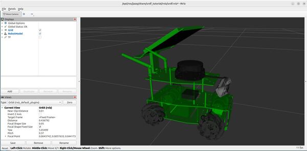
The core macro definition starts with configurable parameters that let you customize how the IMU is attached to your robot:
<xacro:macro name="imu_sensor" params="
    prefix:=''
    parent:='base_link'
    frame_id:='imu'
    xyz_offset:='0 0 0'
    rpy_offset:='0 0 0'
    ...
The physical properties of the IMU are carefully defined to match real-world characteristics. The sensor weighs 31 grams (0.031 kg) and measures approximately 39mm × 38mm × 13mm. It updates its measurements 15 times per second (15 Hz) and is rendered in a dark black color to match typical IMU hardware.
One of the most interesting parts is how the code calculates the moment of inertia – a measure of how hard it is to rotate the sensor around different axes:
<xacro:property name="ixx" value="${(mass/12.0) * (height*height + width*width)}" />
<xacro:property name="iyy" value="${(mass/12.0) * (length*length + height*height)}" />
<xacro:property name="izz" value="${(mass/12.0) * (length*length + width*width)}" />
These calculations come from physics equations for rectangular objects. The 1/12 factor appears because of how mass is distributed in a rectangular shape. Each axis needs different calculations because rotating a rectangular object requires different amounts of force depending on which way you’re turning it.
The visual representation keeps things simple with a basic black box shape:
<visual>
    <origin xyz="0 0 0" rpy="0 0 0"/>
    <geometry>
        <box size="${length} ${width} ${height}"/>
    </geometry>
    <material name="${material_name}">
        <color rgba="${material_color}"/>
    </material>
</visual>
The IMU attaches to your robot using a fixed joint, meaning it doesn’t move relative to whatever part of the robot you attach it to:
<joint name="${prefix}${frame_id}_joint" type="fixed">
    <parent link="${prefix}${parent}"/>
    <child link="${prefix}${frame_id}_link" />
    <origin xyz="${xyz_offset}" rpy="${rpy_offset}"/>
</joint>
The Gazebo simulation settings at the end define how the IMU behaves in the virtual world:
<gazebo reference="${prefix}${frame_id}_link">
    <sensor name="${prefix}imu_sensor" type="imu">
        <topic>${prefix}${topic_name}</topic>
        <update_rate>${update_rate}</update_rate>
        <always_on>${always_on}</always_on>
        <visualize>${visualize}</visualize>
        <gz_frame_id>${prefix}${frame_id}_link</gz_frame_id>
    </sensor>
</gazebo>
This section tells Gazebo to create a virtual IMU sensor that publishes its data to a ROS topic named “imu/data” by default. The sensor stays on continuously during simulation and updates 15 times per second. The visualization is turned off by default since you typically don’t need to see sensor data graphics during simulation.
lidar.urdf.xacro
This file defines a LIDAR (Light Detection and Ranging) sensor for robot simulation in ROS, specifically modeling an RPLidar S2. A LIDAR sensor spins around and uses laser beams to measure distances to objects, creating a 2D map of its surroundings.
The macro starts by defining the physical and operational characteristics of the LIDAR:
<xacro:macro name="lidar_sensor" params="
    prefix:=''
    parent:='base_link'
    frame_id:='laser_frame'
    mesh_file:='file://$(find yahboom_rosmaster_description)/meshes/rplidar/rplidar_s2.stl'
    xyz_offset:='0 0 0.0825'
    ...
The physical properties match a real RPLidar S2 with a width of 77mm diameter, height of 39.8mm, and mass of 185 grams. Like most LIDAR sensors, it’s rendered in black to match the real hardware.
The sensor’s moment of inertia calculations treat the LIDAR as a cylinder:
<xacro:property name="radius" value="${lidar_width/2}" />
<xacro:property name="ixx_iyy" value="${(mass/12) * (3 * radius * radius + lidar_height * lidar_height)}" />
<xacro:property name="izz" value="${(mass/2) * (radius * radius)}" />
The visual appearance uses a detailed 3D model scaled down from millimeters to meters:
<visual>
    <origin xyz="${mesh_xyz_offset}" rpy="${mesh_rpy_offset}"/>
    <geometry>
        <mesh filename="${mesh_file}" scale="${mesh_scale}"/>
    </geometry>
    <material name="${material_name}">
        <color rgba="${material_color}"/>
    </material>
</visual>
The most interesting part is the LIDAR sensor configuration in Gazebo:
<sensor name="${prefix}lidar_sensor" type="gpu_lidar">
    <topic>${prefix}${topic_name}</topic>
    <update_rate>${update_rate}</update_rate>
    <ray>
        <scan>
            <horizontal>
                <samples>${ray_count}</samples>
                <resolution>1</resolution>
                <min_angle>${min_angle}</min_angle>
                <max_angle>${max_angle}</max_angle>
            </horizontal>
This LIDAR simulates a full 360-degree scan (from -π to π radians) with 360 individual laser beams, taking 10 scans per second. It can measure distances from 5cm to 30 meters with a resolution of 13mm, and uses GPU acceleration for better performance.
The sensor is configured as a 2D LIDAR, meaning it scans in a single plane. This is clear from the vertical configuration:
<vertical>
    <samples>1</samples>
    <resolution>1</resolution>
    <min_angle>0</min_angle>
    <max_angle>0</max_angle>
</vertical>
The sensor publishes its data to a ROS topic called “scan” and runs continuously during simulation. The GPU acceleration means it uses your computer’s graphics card to process the laser measurements, making the simulation more efficient.
The physical mounting is handled by a fixed joint that typically places the LIDAR about 8.25cm above its parent link:
<joint name="${prefix}${frame_id}_joint" type="fixed">
    <parent link="${prefix}${parent}"/>
    <child link="${prefix}${frame_id}" />
    <origin xyz="${xyz_offset}" rpy="${rpy_offset}"/>
</joint>
When you use this macro in your robot description, you get a realistic LIDAR sensor that creates accurate distance measurements in a 360-degree field of view. It updates 10 times per second, has realistic physical properties for simulation, uses GPU acceleration for efficient processing, and publishes data in the standard ROS laser scan format.
The data from this simulated LIDAR works just like a real LIDAR for navigation, mapping, obstacle avoidance, and localization tasks in your robotics applications.
rosmaster_x3.urdf.xacro
This is the main assembly file for the ROSMASTER X3 robot. Think of it as a blueprint that brings together all the individual components we looked at earlier into a complete robot. Let’s walk through how this file builds the robot piece by piece.
First, it sets up some basic information:
<?xml version="1.0"?>
<robot xmlns:xacro="http://www.ros.org/wiki/xacro" name="rosmaster_x3">
    <xacro:property name="M_PI" value="3.1415926535897931" />
    <xacro:arg name="prefix" default=""/>
The prefix argument lets you create multiple robots in the same simulation by giving each one a unique name prefix.
Next, it imports all the component descriptions we’ve looked at:
<xacro:include filename="$(find yahboom_rosmaster_description)/urdf/mech/rosmaster_x3_base.urdf.xacro"/>
<xacro:include filename="$(find yahboom_rosmaster_description)/urdf/mech/mecanum_wheel.urdf.xacro"/>
<xacro:include filename="$(find yahboom_rosmaster_description)/urdf/sensors/rgbd_camera.urdf.xacro"/>
<xacro:include filename="$(find yahboom_rosmaster_description)/urdf/sensors/lidar.urdf.xacro"/>
<xacro:include filename="$(find yahboom_rosmaster_description)/urdf/sensors/imu.urdf.xacro"/>
Then it starts assembling the robot. First comes the base:
<xacro:rosmaster_x3_base prefix="$(arg prefix)"/>
Next, it adds the four mecanum wheels. Notice how it uses x_reflect and y_reflect to position each wheel correctly:
<xacro:mecanum_wheel
  prefix="$(arg prefix)"
  side="front_left"
  x_reflect="1"
  y_reflect="1"/>

<xacro:mecanum_wheel
  prefix="$(arg prefix)"
  side="front_right"
  x_reflect="1"
  y_reflect="-1"/>
The reflect values work like this:
- Front wheels have x_reflect=”1″ because they’re at the front
- Back wheels have x_reflect=”-1″ because they’re at the back
- Left wheels have y_reflect=”1″
- Right wheels have y_reflect=”-1″
Then it adds the RGBD camera (like a RealSense):
<xacro:rgbd_camera
  prefix="$(arg prefix)"
  camera_name="cam_1"
  xyz_offset="0.105 0 0.05"
  rpy_offset="0 -0.50 0"/>
The camera is positioned 10.5cm forward, 5cm up, and tilted down slightly (0.5 radians) to see the ground in front of the robot.
The LIDAR sensor comes next:
<xacro:lidar_sensor
  prefix="$(arg prefix)"
  parent="base_link"
  frame_id="laser_frame"
  xyz_offset="0 0 0.0825"
  rpy_offset="0 0 0"/>
It’s mounted 8.25cm above the base, perfectly level to scan the horizontal plane around the robot.
Finally, it adds the IMU sensor:
<xacro:imu_sensor
  prefix="$(arg prefix)"
  parent="base_link"
  frame_id="imu"
  xyz_offset="0 0 0.006"
  rpy_offset="0 0 0"/>
The IMU sits very close to the base (0.6cm up) because it needs to measure the robot’s core movement.
This assembly creates a mobile robot that can:
- Move in any direction using its mecanum wheels
- See objects and depth with its RGBD camera
- Scan its surroundings with the LIDAR
- Track its movement and orientation with the IMU
All these sensors work together – the LIDAR maps the space, the camera identifies objects, and the IMU helps keep track of the robot’s position and movement. The mecanum wheels then let it navigate precisely through its environment.
Build the Package
Now let’s build the package.
buildVisualize the URDF File
Let’s see the URDF file in RViz.
By the way, before you run the command below, be sure to comment out these lines in your XACRO since we haven’t yet got to control with Gazebo.
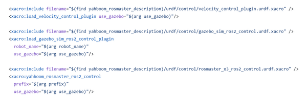
Launch the URDF file. The conversion from XACRO to URDF happens behind the scenes. Be sure to have the correct path to your XACRO file.
ros2 launch urdf_tutorial display.launch.py model:=/home/ubuntu/ros2_ws/src/yahboom_rosmaster/yahboom_rosmaster_description/urdf/robots/rosmaster_x3.urdf.xacro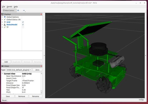
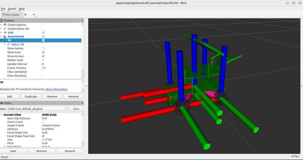
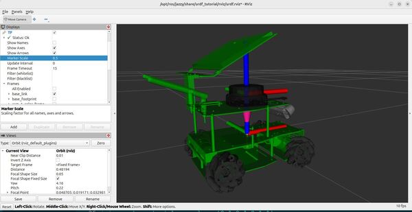
By convention, the red axis is the x-axis, the green axis in the y-axis, and the blue axis is the z-axis.
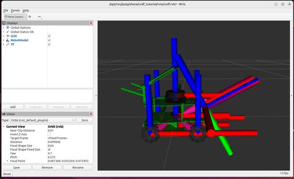
Uncheck the TF checkbox to turn off the axes.
You can use the Joint State Publisher GUI pop-up window to move the links around.
On the left panel under Displays, play around by checking and unchecking different options.
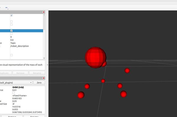
For example, under Robot Model, you can see how the mass is distributed for the robot arm by unchecking “Visual Enabled” and “Collision Enabled” and checking the “Mass” checkbox under “Mass Properties”.
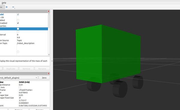
You can also see what simulation engines will use to detect collisions when the mobile robot is commanded to go to a certain point.
Uncheck “Visual Enabled” under Robot Model and check “Collision Enabled.”
You can also see the coordinate frames.
Open a new terminal window, and type the following commands:
cd ~/Documents/ros2 run tf2_tools view_framesTo see the coordinate frames, type:
direvince frames_YYYY-MM-DD_HH.MM.SS.pdf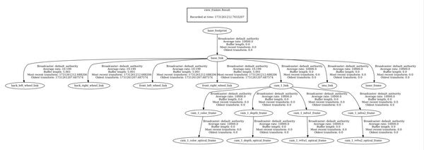
To close RViz, press CTRL + C.
So we can quickly visualize our robot in the future, let’s add a bash command that will enable us to quickly see our URDF.
echo "alias yahboom='ros2 launch urdf_tutorial display.launch.py model:=/home/ubuntu/ros2_ws/src/yahboom_rosmaster/yahboom_rosmaster_description/urdf/robots/rosmaster_x3.urdf.xacro'" >> ~/.bashrc
To see it was added, type:
cat ~/.bashrcsource ~/.bashrcGoing forward, if you want to see your URDF file, type this command in the terminal window:
yahboomThat’s it. Keep building, and I will see you in the next tutorial!

