Winnow2 Algorithm From Scratch | Machine Learning

In this post, I will walk you through the Winnow2 machine learning algorithm, step-by-step. We will develop the code for the algorithm from scratch using Python. We will then run the algorithm on a real-world data set, the breast cancer data set from the UCI Machine Learning Repository. Our goal is to be able to predict if a patient has breast cancer or not based on ten different attributes. Without further ado, let’s get started!

Table of Contents

What is the Winnow2 Algorithm?

The Winnow2 algorithm was invented by Nick Littlestone in the late 1980s. Winnow2 is an example of supervised learning. Supervised learning is the most common type of machine learning.

In supervised learning, you feed the machine learning algorithm data that contains a set of attributes (also known as x, predictors, inputs, features, etc.) and the corresponding classification (also known as label, output, target variable, correct answer, etc.). Each instance (also known as data point, example, etc.) helps the Learner (the prediction mathematical model we are trying to build) learn the association between the attributes and the class. The job of the Learner is to create a model that enables it to use just the values of the attributes to predict the class.

For example, consider how a supervised learning algorithm would approach the breast cancer data set that has 699 instances. Each instance is a different medical patient case seen by a doctor.

winnow2-algorithm-1

For each instance, we have:

  • 9 attributes: clump thickness, uniformity of cell size, uniformity of cell shape, marginal adhesion, single epithelial cell size, bare nuclei, bland chromatin, normal nucleoli, and mitoses.
  • 2 classes: malignant (breast cancer detected) or benign (breast cancer not detected)

The end goal of a classification supervised learning algorithm like Winnow2 is to develop a model that can accurately predict if a new patient has breast cancer or not based on his or her attribute values. And in order to do that, the Learner must be trained on the existing data set in order to learn the association between the 9 attributes and the class.

In Winnow2, we need to preprocess a data set so that both the attributes and the class are binary values, 0 (zero) or 1 (one). For example, in the example I presented above, the class value for each instance is either 0 (benign – breast cancer not detected) or 1 (malignant – breast cancer detected).

Return to Table of Contents

Algorithm Steps

The Winnow2 algorithm continuously updates as each new instance arrives (i.e. an online learning algorithm). Here is how Winnow2 works on a high level:

Step 1: Learner (prediction model) receives an instance (data point):

Since Winnow2 can only work with 0s and 1s, the attribute values need to have already been preprocessed to be either 0 or 1. For example, using the breast cancer data example, attributes like clump thickness need to first be binarized so that they are either 0 or 1. One-hot encoding is the method used in this project in order to perform this binarization.

Step 2: Learner makes a prediction of the class the instance belongs to based on the values of the attributes in the instance

For example, does the Learner believe the patient belongs to the breast cancer class based on the values of the attributes? The Learner predicts 0 if no (benign) or 1 if yes (malignant).

Step 3: Is the Prediction Correct?

The Learner is told the correct class after it makes a prediction. If the learner is correct, nothing happens. Learning (i.e. amending the mathematical model) only occurs when the Learner gets an incorrect answer.

There are two ways for the prediction to be incorrect:

winnow2-algorithm-5

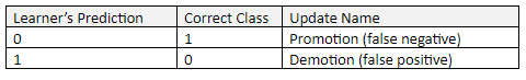
In order to “learn”, a process called “Promotion” (to be explained in the next section) takes place when the Learner incorrectly predicts 0. This situation is a “false negative” result. A false negative occurs when the Learner predicts a person does not have a disease or condition when the person actually does have it.

“Demotion” takes place when the Learner incorrectly predicts 1. This situation is a “false positive” result. A false positive (also known as “false alarm”) occurs when the Learner predicts a person has a specific disease or condition when the person actually does not have it.

Promotion and Demotion: Building the Prediction Model One Instance at a Time

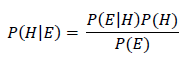
To understand the promotion and demotion activities of Winnow2, we need to first examine the Learner’s mathematical model, the tool being used to predict whether an instance belongs to the benign (0) class or malignant (1) class.

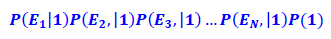
When the Learner receives an instance (“Step 1” from the previous section), it runs the attributes through the following weighted sum:
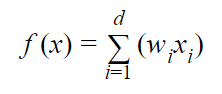
winnow2-algorithm-6

where:

  • d is the total number of attributes
  • wi is the weighting of the ith attribute  
  • xi is the value of the ith attribute in binary format
  • f(x) is the weighted sum (e.g. w1x1 + w2x2 + w3x3 + …. + wdxd)

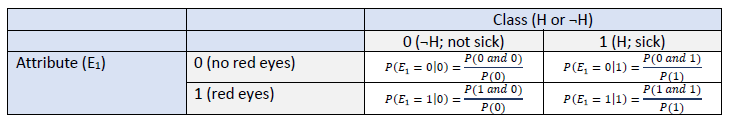
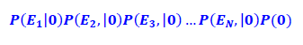
The Learner then predicts an instance’s class (e.g. 1 for malignant and 0 for benign in our breast cancer example) as follows where:

hofx
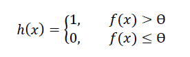
  • h(x) is the predicted class
  • Ɵ is a constant threshold (commonly set to 0.5)

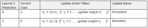
As mentioned before, if the learner makes an incorrect prediction, either promotion or demotion occurs. In both promotion and demotion, the weights wi are modified by using a constant parameter α which is any value greater than 1 (commonly set to 2).

Initially all the weights wi for each attribute are set to 1. They are then adjusted as follows:

winnow2-algorithm-2

Return to Table of Contents

Winnow2 Example Using Real Data

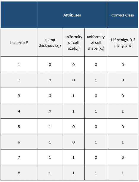
Let’s take a look at the Winnow2 algorithm using an example with real data. We have three different attributes (which have already been converted from real numbers into binary form) and a class variable (which has also been converted into binary form). Our goal is to develop a model that can use just those three attributes to predict if a medical patient has breast cancer or not.

  • 3 attributes: clump thickness (x1), uniformity of cell size(x2), uniformity of cell shape (x3),
  • 2 classes (labels): malignant (breast cancer detected) or benign (breast cancer not detected)

Remember:

  • All weights w for each attribute are initially set to 1. This is known as the “weight vector.”
  • Ɵ = 0.5. This is our threshold.
  • α = 2
  • d = 3 because there are 3 attributes.

Here is the original data set with the attributes (inputs) and the class (output):

winnow2-algorithm-3

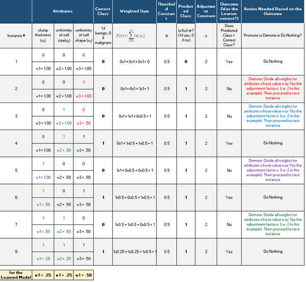
Here is what we have after we run Winnow2. We proceeded row-by-row in the original data set (one instance at a time), which generated this table:

winnow2-algorithm-4

Return to Table of Contents

Winnow2 Implementation

I implemented Winnow2 from scratch in Python and then ran the algorithm on a real-world data set, the breast cancer data set from the UCI Machine Learning Repository.

Preprocessing the Example Data Set – Breast Cancer

The breast cancer data set contains 699 instances, 10 attributes, and a class – malignant or benign. I transformed the attributes and classes into binary numbers (making them discrete is fine too, but they cannot be continuous) so that the algorithms could process the data properly and efficiently. If attribute value was greater than 5, the value was changed to 1, otherwise it was 0. I also changed Benign from 2 to 0 and Malignant from 4 to 1.

There were 16 missing attribute values in the data set, each denoted with a “?”. I chose a random number between 1 and 10 (inclusive) to fill in the data.

Finally, for each run, data sets were split into 67% for training and 33% for testing. Summary statistics were then calculated.

Here is the format the input data needs to take in the raw text/csv file. Attributes can be numerical or text, but in this example the were all numerical:

Columns (0 through N)

  • 0: Instance ID
  • 1: Attribute 1 (in binary)
  • 2: Attribute 2 (in binary)
  • 3: Attribute 3 (in binary)
  • N: Actual Class (in binary)

The program then adds 8 additional columns:

  • N + 1: Weighted Sum (of the attributes)
  • N + 2: Predicted Class (in binary)…Weighted Sum > 0? (1 if yes; 0 if no)
  • N + 3: True Positive (1 if yes; O if no)
  • N + 4: False Positive (1 if yes; 0 if no)
  • N + 5: False Negative (1 if yes; 0 if no)
  • N + 6: True Negative (1 if yes; 0 if no)
  • N + 7: Promote (1 if yes; 0 if no)  [for training set only]
  • N + 8: Demote (1 if yes; 0 if no) [for training set only]

Here is a link to the input file after all that preprocessing was performed.

Here is a link to the output file after the algorithm below was run on the input file.

Here is a link to the final weights after the algorithm below was run on the input file.

Return to Table of Contents

Winnow2 Algorithm in Python, Coded From Scratch

Here is the code. Don’t be scared at how long the code is. I included a bunch of comments so that you know what is going on at each step. I recommend you copy and paste all this code into your favorite IDE. If there is a term or a piece of code that you have never seen before, look it up on Google (even the pros who have been at this a long time have to look things up on Google all the time! This is how you learn).

import pandas as pd # Import Pandas library 
import numpy as np # Import Numpy library

# File name: winnow2.py
# Author: Addison Sears-Collins
# Date created: 5/31/2019
# Python version: 3.7
# Description: Implementation of the Winnow2 machine learning
# algorithm invented by Nick Littlestone. Used for 2-class classificaiton
# problems (e.g. cancer/no cancer....spam/not spam, etc...)
# Nick Littlestone (1988). "Learning Quickly When Irrelevant Attributes 
# Abound: A New Linear-threshold Algorithm", Machine Learning 285–318(2)

# Required Data Set Format:
# Columns (0 through N)
# 0: Instance ID
# 1: Attribute 1 (in binary)
# 2: Attribute 2 (in binary)
# 3: Attribute 3 (in binary)
# ...
# N: Actual Class (in binary)

# This program then adds 8 additional columns:
# N + 1: Weighted Sum (of the attributes)
# N + 2: Predicted Class (in binary)...Weighted Sum > 0? (1 if yes; 0 if no)
# N + 3: True Positive (1 if yes; O if no)
# N + 4: False Positive (1 if yes; 0 if no)
# N + 5: False Negative (1 if yes; 0 if no)
# N + 6: True Negative (1 if yes; 0 if no)
# N + 7: Promote (1 if yes; 0 if no) [for training set only]
# N + 8: Demote (1 if yes; 0 if no)  [for training set only]

################ INPUT YOUR OWN VALUES IN THIS SECTION ######################
ALGORITHM_NAME = "Winnow2"
THETA = 0.5   # This is the threshold constant for the Winnow2 algorithm
ALPHA = 2.0    # This is the adjustment constant for promotion & demotion
DATA_PATH = "breast_cancer_dataset.txt"  # Directory where data set is located
TRAIN_WEIGHTS_FILE = "breast_cancer_winnow2_train_weights.txt" # Weights of learned model
TRAIN_OUT_FILE = "breast_cancer_winnow2_train_out.txt" # Training phase of the model
TEST_STATS_FILE = "breast_cancer_winnow2_test_stats.txt" # Testing statistics
TEST_OUT_FILE = "breast_cancer_winnow2_test_out.txt" # Testing phase of the model
SEPARATOR = ","  # Separator for the data set (e.g. "\t" for tab data)
CLASS_IF_ONE = "Malignant" # If Class value is 1 (e.g. Malignant, Spam, etc.)
CLASS_IF_ZERO = "Benign"  # If Class value is 0 (e.g. Benign, Not Spam, etc.)
TRAINING_DATA_PRCT = 0.67 # % of data set used for training
testing_data_prct = 1 - TRAINING_DATA_PRCT # % of data set used for testing
SEED = 99  # SEED for the random number generator. Default: 99
#############################################################################

# Read a text file and store records in a Pandas dataframe
pd_data = pd.read_csv(DATA_PATH, sep=SEPARATOR)

# Create a training dataframe by sampling random instances from original data.
# random_state guarantees that the pseudo-random number generator generates 
# the same sequence of random numbers each time.
pd_training_data = pd_data.sample(frac=TRAINING_DATA_PRCT, random_state=SEED)

# Create a testing dataframe. Dropping the training data from the original
# dataframe ensures training and testing dataframes have different instances
pd_testing_data = pd_data.drop(pd_training_data.index)

# Convert training dataframes to Numpy arrays
np_training_data = pd_training_data.values
np_testing_data = pd_testing_data.values

#np_training_data = pd_data.values # Used for testing only
#np_testing_data = pd_data.values  # Used for testing only

################ Begin Training Phase #####################################

# Calculate the number of instances, columns, and attributes in the data set
# Assumes 1 column for the instance ID and 1 column for the class
# Record the index of the column that contains the actual class
no_of_instances = np_training_data.shape[0]
no_of_columns = np_training_data.shape[1]
no_of_attributes = no_of_columns - 2
actual_class_column = no_of_columns - 1

# Initialize the weight vector. Initialize all weights to 1.
# First column of weight vector is not used (i.e. Instance ID)
weights = np.ones(no_of_attributes + 1)

# Create a new array that has 8 columns, initialized to 99 for each value
extra_columns_train = np.full((no_of_instances, 8),99)

# Add extra columns to the training data set
np_training_data = np.append(np_training_data, extra_columns_train, axis=1)

# Make sure it is an array of floats
np_training_data = np_training_data.astype(float)

# Build the learning model one instance at a time
for row in range(0, no_of_instances):

    # Set the weighted sum to 0
    weighted_sum = 0

    # Calculate the weighted sum of the attributes
    for col in range(1, no_of_attributes + 1):
        weighted_sum += (weights[col] * np_training_data[row,col])

    # Record the weighted sum into column N + 1, the column just to the right
    # of the actual class column
    np_training_data[row, actual_class_column + 1] = weighted_sum

    # Set the predicted class to 99
    predicted_class = 99

    # Learner's prediction: Is the weighted sum > THETA?
    if weighted_sum > THETA:
        predicted_class = 1
    else:
        predicted_class = 0

    # Record the predicted class into column N + 2
    np_training_data[row, actual_class_column + 2] = predicted_class

    # Record the actual class into a variable
    actual_class = np_training_data[row, actual_class_column]

    # Initialize the prediction outcomes
    # These variables are standard inputs into a "Confusion Matrix"
    true_positive = 0   # Predicted class = 1; Actual class = 1 (hit)
    false_positive = 0  # Predicted class = 1; Actual class = 0 (false alarm)
    false_negative = 0  # Predicted class = 0; Actual class = 1 (miss)
    true_negative = 0   # Predicted class = 0; Actual class = 0 

    # Determine the outcome of the Learner's prediction
    if predicted_class == 1 and actual_class == 1:
        true_positive = 1
    elif predicted_class == 1 and actual_class == 0:
        false_positive = 1
    elif predicted_class == 0 and actual_class == 1:
        false_negative = 1
    else:
        true_negative = 1

    # Record the outcome of the Learner's prediction
    np_training_data[row, actual_class_column + 3] = true_positive
    np_training_data[row, actual_class_column + 4] = false_positive
    np_training_data[row, actual_class_column + 5] = false_negative
    np_training_data[row, actual_class_column + 6] = true_negative

    # Set the promote and demote variables to 0
    promote = 0
    demote = 0

    # Promote if false negative
    if false_negative == 1:
        promote = 1
   
    # Demote if false positive
    if false_positive == 1:
        demote = 1

    # Record if either a promotion or demotion is needed
    np_training_data[row, actual_class_column + 7] = promote
    np_training_data[row, actual_class_column + 8] = demote

    # Run through each attribute and see if it is equal to 1
    # If attribute is 1, we need to either demote or promote (adjust the
    # corresponding weight by ALPHA).
    if demote == 1:
        for col in range(1, no_of_attributes + 1):
            if(np_training_data[row,col] == 1):
                weights[col] /= ALPHA
    if promote == 1:
        for col in range(1, no_of_attributes + 1):
            if(np_training_data[row,col] == 1):
                weights[col] *= ALPHA

# Open a new file to save the weights
outfile1 = open(TRAIN_WEIGHTS_FILE,"w") 

# Write the weights of the Learned model to a file
outfile1.write("----------------------------------------------------------\n")
outfile1.write(" " + ALGORITHM_NAME + " Training Weights\n")
outfile1.write("----------------------------------------------------------\n")
outfile1.write("Data Set : " + DATA_PATH + "\n")
outfile1.write("\n----------------------------\n")
outfile1.write("Weights of the Learned Model\n")
outfile1.write("----------------------------\n")
for col in range(1, no_of_attributes + 1):
    colname = pd_training_data.columns[col]
    s = str(weights[col])
    outfile1.write(colname + " : " + s + "\n")

# Write the relevant constants used in the model to a file
outfile1.write("\n")
outfile1.write("-----------\n")
outfile1.write("Constants\n")
outfile1.write("-----------\n")
s = str(THETA)
outfile1.write("THETA = " + s + "\n")
s = str(ALPHA)
outfile1.write("ALPHA = " + s + "\n")

# Close the weights file
outfile1.close()

# Print the weights of the Learned model
print("----------------------------------------------------------")
print(" " + ALGORITHM_NAME + " Results")
print("----------------------------------------------------------")
print("Data Set : " + DATA_PATH)
print()
print()
print("----------------------------")
print("Weights of the Learned Model")
print("----------------------------")
for col in range(1, no_of_attributes + 1):
    colname = pd_training_data.columns[col]
    s = str(weights[col])
    print(colname + " : " + s)

# Print the relevant constants used in the model
print()
print()
print("-----------")
print("Constants")
print("-----------")
s = str(THETA)
print("THETA = " + s)
s = str(ALPHA)
print("ALPHA = " + s)
print()

# Print the learned model runs in binary form
print("-------------------------------------------------------")
print("Learned Model Runs of the Training Data Set (in binary)")
print("-------------------------------------------------------")
print(np_training_data)
print()
print()

# Convert Numpy array to a dataframe
df = pd.DataFrame(data=np_training_data)

# Replace 0s and 1s in the attribute columns with False and True
for col in range(1, no_of_attributes + 1):
    df[[col]] = df[[col]].replace([0,1],["False","True"])

# Replace values in Actual Class column with more descriptive values
df[[actual_class_column]] = df[[actual_class_column]].replace([0,1],[CLASS_IF_ZERO,CLASS_IF_ONE])

# Replace values in Predicted Class column with more descriptive values
df[[actual_class_column + 2]] = df[[actual_class_column + 2]].replace([0,1],[CLASS_IF_ZERO,CLASS_IF_ONE])

# Change prediction outcomes to more descriptive values
for col in range(actual_class_column + 3,actual_class_column + 9):
    df[[col]] = df[[col]].replace([0,1],["No","Yes"])

# Rename the columns
df.rename(columns={actual_class_column + 1 : "Weighted Sum" }, inplace = True)
df.rename(columns={actual_class_column + 2 : "Predicted Class" }, inplace = True)
df.rename(columns={actual_class_column + 3 : "True Positive" }, inplace = True)
df.rename(columns={actual_class_column + 4 : "False Positive" }, inplace = True)
df.rename(columns={actual_class_column + 5 : "False Negative" }, inplace = True)
df.rename(columns={actual_class_column + 6 : "True Negative" }, inplace = True)
df.rename(columns={actual_class_column + 7 : "Promote" }, inplace = True)
df.rename(columns={actual_class_column + 8 : "Demote" }, inplace = True)

# Change remaining columns names from position numbers to descriptive names
for pos in range(0,actual_class_column + 1):
    df.rename(columns={pos : pd_data.columns[pos] }, inplace = True)

print("-------------------------------------------------------")
print("Learned Model Runs of the Training Data Set (readable) ")
print("-------------------------------------------------------")
# Print the revamped dataframe
print(df)

# Write revamped dataframe to a file
df.to_csv(TRAIN_OUT_FILE, sep=",", header=True)
################ End Training Phase #####################################

################ Begin Testing Phase ######################################

# Calculate the number of instances, columns, and attributes in the data set
# Assumes 1 column for the instance ID and 1 column for the class
# Record the index of the column that contains the actual class
no_of_instances = np_testing_data.shape[0]
no_of_columns = np_testing_data.shape[1]
no_of_attributes = no_of_columns - 2
actual_class_column = no_of_columns - 1

# Create a new array that has 6 columns, initialized to 99 for each value
extra_columns_test = np.full((no_of_instances, 6),99)

# Add extra columns to the testing data set
np_testing_data = np.append(np_testing_data, extra_columns_test, axis=1)

# Make sure it is an array of floats
np_testing_data = np_testing_data.astype(float)

# Test the learning model one instance at a time
for row in range(0, no_of_instances):

    # Set the weighted sum to 0
    weighted_sum = 0

    # Calculate the weighted sum of the attributes
    for col in range(1, no_of_attributes + 1):
        weighted_sum += (weights[col] * np_testing_data[row,col])

    # Record the weighted sum into column N + 1, the column just to the right
    # of the actual class column
    np_testing_data[row, actual_class_column + 1] = weighted_sum

    # Set the predicted class to 99
    predicted_class = 99

    # Learner's prediction: Is the weighted sum > THETA?
    if weighted_sum > THETA:
        predicted_class = 1
    else:
        predicted_class = 0

    # Record the predicted class into column N + 2
    np_testing_data[row, actual_class_column + 2] = predicted_class

    # Record the actual class into a variable
    actual_class = np_testing_data[row, actual_class_column]

    # Initialize the prediction outcomes
    # These variables are standard inputs into a "Confusion Matrix"
    true_positive = 0   # Predicted class = 1; Actual class = 1 (hit)
    false_positive = 0  # Predicted class = 1; Actual class = 0 (false alarm)
    false_negative = 0  # Predicted class = 0; Actual class = 1 (miss)
    true_negative = 0   # Predicted class = 0; Actual class = 0 

    # Determine the outcome of the Learner's prediction
    if predicted_class == 1 and actual_class == 1:
        true_positive = 1
    elif predicted_class == 1 and actual_class == 0:
        false_positive = 1
    elif predicted_class == 0 and actual_class == 1:
        false_negative = 1
    else:
        true_negative = 1

    # Record the outcome of the Learner's prediction
    np_testing_data[row, actual_class_column + 3] = true_positive
    np_testing_data[row, actual_class_column + 4] = false_positive
    np_testing_data[row, actual_class_column + 5] = false_negative
    np_testing_data[row, actual_class_column + 6] = true_negative

# Convert Numpy array to a dataframe
df = pd.DataFrame(data=np_testing_data)

# Replace 0s and 1s in the attribute columns with False and True
for col in range(1, no_of_attributes + 1):
    df[[col]] = df[[col]].replace([0,1],["False","True"])

# Replace values in Actual Class column with more descriptive values
df[[actual_class_column]] = df[[actual_class_column]].replace([0,1],[CLASS_IF_ZERO,CLASS_IF_ONE])

# Replace values in Predicted Class column with more descriptive values
df[[actual_class_column + 2]] = df[[actual_class_column + 2]].replace([0,1],[CLASS_IF_ZERO,CLASS_IF_ONE])

# Change prediction outcomes to more descriptive values
for col in range(actual_class_column + 3,actual_class_column + 7):
    df[[col]] = df[[col]].replace([0,1],["No","Yes"])

# Rename the columns
df.rename(columns={actual_class_column + 1 : "Weighted Sum" }, inplace = True)
df.rename(columns={actual_class_column + 2 : "Predicted Class" }, inplace = True)
df.rename(columns={actual_class_column + 3 : "True Positive" }, inplace = True)
df.rename(columns={actual_class_column + 4 : "False Positive" }, inplace = True)
df.rename(columns={actual_class_column + 5 : "False Negative" }, inplace = True)
df.rename(columns={actual_class_column + 6 : "True Negative" }, inplace = True)

df_numerical = pd.DataFrame(data=np_testing_data) # Keep the values in this dataframe numerical
df_numerical.rename(columns={actual_class_column + 3 : "True Positive" }, inplace = True)
df_numerical.rename(columns={actual_class_column + 4 : "False Positive" }, inplace = True)
df_numerical.rename(columns={actual_class_column + 5 : "False Negative" }, inplace = True)
df_numerical.rename(columns={actual_class_column + 6 : "True Negative" }, inplace = True)

# Change remaining columns names from position numbers to descriptive names
for pos in range(0,actual_class_column + 1):
    df.rename(columns={pos : pd_data.columns[pos] }, inplace = True)

print("-------------------------------------------------------")
print("Learned Model Predictions on Testing Data Set")
print("-------------------------------------------------------")
# Print the revamped dataframe
print(df)

# Write revamped dataframe to a file
df.to_csv(TEST_OUT_FILE, sep=",", header=True)

# Open a new file to save the summary statistics
outfile2 = open(TEST_STATS_FILE,"w") 

# Write to a file
outfile2.write("----------------------------------------------------------\n")
outfile2.write(ALGORITHM_NAME + " Summary Statistics (Testing)\n")
outfile2.write("----------------------------------------------------------\n")
outfile2.write("Data Set : " + DATA_PATH + "\n")

# Write the relevant stats to a file
outfile2.write("\n")
outfile2.write("Number of Test Instances : " + 
    str(np_testing_data.shape[0])+ "\n")

tp = df_numerical["True Positive"].sum()
s = str(int(tp))
outfile2.write("True Positives : " + s + "\n")

fp = df_numerical["False Positive"].sum()
s = str(int(fp))
outfile2.write("False Positives : " + s + "\n")

fn = df_numerical["False Negative"].sum()
s = str(int(fn))
outfile2.write("False Negatives : " + s + "\n")

tn = df_numerical["True Negative"].sum()
s = str(int(tn))
outfile2.write("True Negatives : " + s + "\n")

accuracy = (tp + tn)/(tp + tn + fp + fn)
accuracy *= 100
s = str(accuracy)
outfile2.write("Accuracy : " + s + "%\n")

specificity = (tn)/(tn + fp)
specificity *= 100
s = str(specificity)
outfile2.write("Specificity : " + s + "%\n")

precision = (tp)/(tp + fp)
precision *= 100
s = str(precision)
outfile2.write("Precision : " + s + "%\n")

recall = (tp)/(tp + fn)
recall *= 100
s = str(recall)
outfile2.write("Recall : " + s + "%\n")

neg_pred_value = (tn)/(tn + fn)
neg_pred_value *= 100
s = str(neg_pred_value)
outfile2.write("Negative Predictive Value : " + s + "%\n")

miss_rate = (fn)/(fn + tp)
miss_rate *= 100
s = str(miss_rate)
outfile2.write("Miss Rate  : " + s + "%\n")

fall_out = (fp)/(fp + tn)
fall_out *= 100
s = str(fall_out)
outfile2.write("Fall-Out : " + s + "%\n")

false_discovery_rate = (fp)/(fp + tp)
false_discovery_rate *= 100
s = str(false_discovery_rate)
outfile2.write("False Discovery Rate : " + s + "%\n")

false_omission_rate = (fn)/(fn + tn)
false_omission_rate *= 100
s = str(false_omission_rate)
outfile2.write("False Omission Rate  : " + s + "%\n")

f1_score = (2 * tp)/((2 * tp) + fp + fn)
s = str(f1_score)
outfile2.write("F1 Score: " + s)

# Close the weights file
outfile2.close()

# Print statistics to console
print()
print()
print("-------------------------------------------------------")
print(ALGORITHM_NAME + " Summary Statistics (Testing)")
print("-------------------------------------------------------")
print("Data Set : " + DATA_PATH)

# Print the relevant stats to the console
print()
print("Number of Test Instances : " + 
    str(np_testing_data.shape[0]))

s = str(int(tp))
print("True Positives : " + s)

s = str(int(fp))
print("False Positives : " + s)

s = str(int(fn))
print("False Negatives : " + s)

s = str(int(tn))
print("True Negatives : " + s)

s = str(accuracy)
print("Accuracy : " + s + "%")

s = str(specificity)
print("Specificity : " + s + "%")

s = str(precision)
print("Precision : " + s + "%")

s = str(recall)
print("Recall : " + s + "%")

s = str(neg_pred_value)
print("Negative Predictive Value : " + s + "%")

s = str(miss_rate)
print("Miss Rate  : " + s + "%")

s = str(fall_out)
print("Fall-Out : " + s + "%")

s = str(false_discovery_rate)
print("False Discovery Rate : " + s + "%")

s = str(false_omission_rate)
print("False Omission Rate  : " + s + "%")

s = str(f1_score)
print("F1 Score: " + s)


###################### End Testing Phase ######################################

Return to Table of Contents

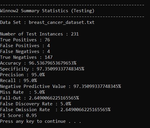
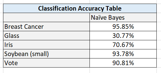
Output Statistics of Winnow2 on the Breast Cancer Data Set

Here is a link to a screenshot of the summary statistics:

breast_cancer_results

Return to Table of Contents

Naive Bayes Algorithm From Scratch | Machine Learning

In this post, I will walk you through the Naive Bayes machine learning algorithm, step-by-step. We will develop the code for the algorithm from scratch using Python. We’ll then run the algorithm on real-world data sets from the UCI Machine Learning Repository. On one of the data sets, we’ll predict if a patient has breast cancer or not based on ten different attributes. Let’s get started!

Table of Contents

What is Naive Bayes?

The Naive Bayes algorithm is a technique based on Bayes Theorem for calculating the probability of a hypothesis (H) given some pieces of evidence (E).

For example, suppose we are trying to identify if a person is sick or not. Our hypothesis is that the person is sick.

nurse_checks_blood_pressure_1

We would naturally take a look at the evidence (eye color, body temperature, blood pressure, etc.) to determine if the person is sick or not. Each piece of evidence provides us clues. From that evidence, we can then use the Naive Bayes algorithm to calculate two probabilities:

  • Probability 1: The probability that the person is sick given she has red eyes, a body temperature of 99°F, and has normal blood pressure.
  • Probability 2: The probability that the person is not sick given she has red eyes, a body temperature of 99°F, and has normal blood pressure.

We then classify the person as being sick or not based on which probability (Probability 1 vs. Probability 2) is the highest.

Mathematically, Bayes theorem can be expressed as follows:

naive-bayes-1

Or in expanded form, we have:

naive-bayes-2

Or…

naive-bayes-3

Where:

  • P = probability
  • | = given
  • E = evidence (e.g. red eyes, body temperature, etc.)
  • H = hypothesis (e.g. sick)
  • ¬ = not
  • P(H|E1, E2,E3,…,EN) = posterior probability: the probability of a hypothesis after taking the evidence into account (e.g. probability of being sick given all this evidence)
  • P(E1, E2,E3,…,EN|H)= likelihood: the probability of the evidence given the hypothesis (e.g. probability of having red eyes given that a person is sick)
  • P(H) = class prior probability: the known probability of the hypothesis (e.g. probability of being sick for the population or entire sample of instances)

The equation above says: “The probability of the hypothesis (e.g. a person is sick) given the evidence (e.g. eye color, body temperature, blood pressure) is equal to the probability of the evidence given the hypothesis times the probability of the hypothesis divided by the probability of the evidence.”

The key assumption with the Bayes theorem is that all of the attributes are conditionally independent. In other words, the occurrence of one piece of evidence gives no information about the probability of another piece of evidence occurring.

For example, Bayes theorem would assume that the probability of having red eyes gives no information about the probability of having a high body temperature. We know this is not often the case. Such an assumption is naive, and that is why we call this classification algorithm the Naive Bayes algorithm.

We can therefore rewrite the equation based on the probability rule of conditional independence, which is:

naive-bayes-4

Bayes equation can be rewritten as:

naive-bayes-5

Return to Table of Contents

Algorithm Steps

Training Phase

Recall in Naive Bayes, for a 2-class classification problem (e.g. sick or not sick), we need to calculate two probabilities for each instance. The highest probability is our prediction.:

Probability 1 (sick): The probability that the person is sick given she has red eyes, a body temperature of 99°F, and has normal blood pressure.

naive-bayes-6-1

Probability 2 (not sick): The probability that the person is not sick given she has red eyes, a body temperature of 99°F, and has a normal blood pressure.

naive-bayes-7

If Probability 1 > Probability 2, she is sick. Otherwise, she is not sick

Notice, the denominators above are both equal. Because they are both equal, we can ignore them for training our model since all we need to do is to compare the numerators.

  • Probability 1 (sick): The probability that the person is sick given she has red eyes, a body temperature of 99°F, and has a normal blood pressure.
naive-bayes-8
  • Probability 2 (not sick): The probability that the person is not sick given she has red eyes, a body temperature of 99°F, and has a normal blood pressure.
naive-bayes-9

This makes our lives easier, since now all Naive Bayes algorithm needs to do to train on a data set is to calculate those values in blue above in order to make a classification prediction (sick or not sick). That is, we need to calculate two class prior probabilities (sick or not sick for the whole sample or population) plus the conditional probability of each unique value in each attribute for each class:

Number of Probabilities Calculated during Training Phase of Naive Bayes = 2 class prior probabilities + 2 * (# of unique values for E1) + 2 * (# of unique values for E2) + … 2 * (# of unique values for EN)

If all pieces of evidence were binary (e.g. red eyes, no red eyes) and the class is binary (sick or not sick), we would need to calculate four probabilities for each attribute. The total number of probabilities calculated in the training phase is therefore (where N is the number of attributes):

Number of Probabilities Calculated during Training Phase of Naive Bayes = 2 + 4N

For example, let’s see all the probabilities that would need to be calculated for binary attribute E1 (e.g. red eyes or no red eyes):

naive-bayes-10

We have our two class prior probabilities. These will be the same for all attributes:

  1. P(1) = (Total number of people that are sick in the training data set) / (Total number of people in the training data set)
  2. P(0) =  (Total number of people that are not sick in the training data set) / (Total number of people in the training data set)

And since (N = number, S = total number of instances in the training data set)…

naive-bayes-11

To complete the table for attribute E1, we calculate four different probabilities:

naive-bayes-12

We have to store these probabilities somewhere so they can be looked up during the testing phase. In my program, I stored them in a Python dictionary, with the following search key: <attribute_name><attribute_value><class_value>.

For example, the search key redeyes01, would return the probability of not having red eyes given someone is sick:

naive-bayes-13

That’s it. Once we have the tables for each attribute along with the class prior probabilities, the algorithm can go to work and make predictions for new instances.

Return to Table of Contents

Testing Phase

Having calculated the required probabilities and stored them somewhere, the algorithm is ready to make its predictions for new instances. As mentioned in the previous section, for each instance (i.e. row of the testing data set), two calculations need to be made and then the results are compared.

1. Probability 1 (sick): The probability that the person is sick given she has red eyes, a body temperature of 99°F, and has normal blood pressure.

naive-bayes-14

2.Probability 2 (not sick): The probability that the person is not sick given she has red eyes, a body temperature of 99°F, and has a normal blood pressure.

naive-bayes-15

3. If Probability 1 > Probability 2, she is sick. Otherwise, she is not sick

4. Proceed to the next instance and repeat 1-3.

Return to Table of Contents

Naive Bayes Implementation

The Naive Bayes algorithm was implemented from scratch. The Breast Cancer, Glass, Iris, Soybean (small), and Vote data sets were preprocessed to meet the input requirements of the algorithms. I used five-fold stratified cross-validation to evaluate the performance of the models.

Required Data Set Format for Naïve Bayes

Columns (0 through N)

  • 0: Instance ID
  • 1: Attribute 1
  • 2: Attribute 2
  • 3: Attribute 3
  • N: Actual Class

The program then adds two additional columns for the testing set.

  • N + 1: Predicted Class
  • N + 2: Prediction Correct? (1 if yes, 0 if no)

Breast Cancer Data Set

This breast cancer data set contains 699 instances, 10 attributes, and a class – malignant or benign (Wolberg, 1992).

Modification of Attribute Values

The actual class value was changed to “Benign” or “Malignant.”

I transformed the attributes into binary numbers so that the algorithms could process the data properly and efficiently. If attribute value was greater than 5, the value was changed to 1, otherwise it was 0.

Missing Data

There were 16 missing attribute values, each denoted with a “?”. I chose a random number between 1 and 10 (inclusive) to fill in the data.

Glass Data Set

This glass data set contains 214 instances, 10 attributes, and 7 classes (German, 1987). The purpose of the data set is to identify the type of glass.

Modification of Attribute Values

If attribute values were greater than the median of the attribute, value was changed to 1, otherwise it was set to 0.

Missing Data

There are no missing values in this data set.

Iris Data Set

This data set contains 3 classes of 50 instances each (150 instances in total), where each class refers to a different type of iris plant (Fisher, 1988).

Modification of Attribute Values

If attribute values were greater than the median of the attribute, value was changed to 1, otherwise it was set to 0.

Missing Data

There were no missing attribute values.

Soybean Data Set (small)

This soybean (small) data set contains 47 instances, 35 attributes, and 4 classes (Michalski, 1980). The purpose of the data set is to determine the disease type.

Modification of Attribute Values

If attribute values were greater than the median of the attribute, value was changed to 1, otherwise it was set to 0.

Missing Data

There are no missing values in this data set.

Vote Data Set

This data set includes votes for each of the U.S. House of Representatives Congressmen (435 instances) on the 16 key votes identified by the Congressional Quarterly Almanac (Schlimmer, 1987). The purpose of the data set is to identify the representative as either a Democrat or Republican.

  • 267 Democrats
  • 168 Republicans

Modification of Attribute Values

I did the following modifications:

  • Changed all “y” to 1 and all “n” to 0.

Missing Data

Missing values were denoted as “?”. To fill in those missing values, I chose random number, either 0 (“No”) or 1 (“Yes”).

Return to Table of Contents

Naive Bayes Algorithm in Python, Coded From Scratch

Here are the input files for the code below:

Here is the driver code that contains the main method. I recommend copying and pasting it into a text editor like Notepad++ or an IDE so that you don’t have to do any horizontal scrolling to see the entire code. The code is long (don’t be scared!), but that is because it includes a ton of notes so that you know what is going on:

import pandas as pd # Import Pandas library 
import numpy as np # Import Numpy library
import five_fold_stratified_cv
import naive_bayes

# File name: naive_bayes_driver.py
# Author: Addison Sears-Collins
# Date created: 7/17/2019
# Python version: 3.7
# Description: Driver for the naive_bayes.py program 
# (Naive Bayes)

# Required Data Set Format for Disrete Class Values
# Columns (0 through N)
# 0: Instance ID
# 1: Attribute 1 
# 2: Attribute 2
# 3: Attribute 3 
# ...
# N: Actual Class

# The naive_bayes.py program then adds 2 additional columns for the test set.
# N + 1: Predicted Class
# N + 2: Prediction Correct? (1 if yes, 0 if no)

ALGORITHM_NAME = "Naive Bayes"
SEPARATOR = ","  # Separator for the data set (e.g. "\t" for tab data)

def main():

    print("Welcome to the " +  ALGORITHM_NAME + " Program!")
    print()

    # Directory where data set is located
    data_path = input("Enter the path to your input file: ") 
    #data_path = "breast_cancer.txt"

    # Read the full text file and store records in a Pandas dataframe
    pd_data_set = pd.read_csv(data_path, sep=SEPARATOR)

    # Show functioning of the program
    trace_runs_file = input("Enter the name of your trace runs file: ") 
    #trace_runs_file = "breast_cancer_naive_bayes_trace_runs.txt"

    # Open a new file to save trace runs
    outfile_tr = open(trace_runs_file,"w") 

    # Testing statistics
    test_stats_file = input("Enter the name of your test statistics file: ") 
    #test_stats_file = "breast_cancer_naive_bayes_test_stats.txt"

    # Open a test_stats_file 
    outfile_ts = open(test_stats_file,"w")

    # The number of folds in the cross-validation
    NO_OF_FOLDS = 5 

    # Generate the five stratified folds
    fold0, fold1, fold2, fold3, fold4 = five_fold_stratified_cv.get_five_folds(
        pd_data_set)

    training_dataset = None
    test_dataset = None

    # Create an empty array of length 5 to store the accuracy_statistics 
    # (classification accuracy)
    accuracy_statistics = np.zeros(NO_OF_FOLDS)

    # Run Naive Bayes the designated number of times as indicated by the 
    # number of folds
    for experiment in range(0, NO_OF_FOLDS):

        print()
        print("Running Experiment " + str(experiment + 1) + " ...")
        print()
        outfile_tr.write("Running Experiment " + str(experiment + 1) + " ...\n")
        outfile_tr.write("\n")

        # Each fold will have a chance to be the test data set
        if experiment == 0:
            test_dataset = fold0
            training_dataset = pd.concat([
               fold1, fold2, fold3, fold4], ignore_index=True, sort=False)                
        elif experiment == 1:
            test_dataset = fold1
            training_dataset = pd.concat([
               fold0, fold2, fold3, fold4], ignore_index=True, sort=False) 
        elif experiment == 2:
            test_dataset = fold2
            training_dataset = pd.concat([
               fold0, fold1, fold3, fold4], ignore_index=True, sort=False) 
        elif experiment == 3:
            test_dataset = fold3
            training_dataset = pd.concat([
               fold0, fold1, fold2, fold4], ignore_index=True, sort=False) 
        else:
            test_dataset = fold4
            training_dataset = pd.concat([
               fold0, fold1, fold2, fold3], ignore_index=True, sort=False) 
        
        # Run Naive Bayes
        accuracy, predictions, learned_model, no_of_instances_test = (
            naive_bayes.naive_bayes(training_dataset,test_dataset))

        # Replace 1 with Yes and 0 with No in the 'Prediction 
        # Correct?' column
        predictions['Prediction Correct?'] = predictions[
            'Prediction Correct?'].map({1: "Yes", 0: "No"})

        # Print the trace runs of each experiment
        print("Accuracy:")
        print(str(accuracy * 100) + "%")
        print()
        print("Classifications:")
        print(predictions)
        print()
        print("Learned Model (Likelihood Table):")
        print(learned_model)
        print()
        print("Number of Test Instances:")
        print(str(no_of_instances_test))
        print() 

        outfile_tr.write("Accuracy:")
        outfile_tr.write(str(accuracy * 100) + "%\n\n")
        outfile_tr.write("Classifications:\n")
        outfile_tr.write(str(predictions) + "\n\n")
        outfile_tr.write("Learned Model (Likelihood Table):\n")
        outfile_tr.write(str(learned_model) + "\n\n")
        outfile_tr.write("Number of Test Instances:")
        outfile_tr.write(str(no_of_instances_test) + "\n\n")

        # Store the accuracy in the accuracy_statistics array
        accuracy_statistics[experiment] = accuracy

    outfile_tr.write("Experiments Completed.\n")
    print("Experiments Completed.\n")

    # Write to a file
    outfile_ts.write("----------------------------------------------------------\n")
    outfile_ts.write(ALGORITHM_NAME + " Summary Statistics\n")
    outfile_ts.write("----------------------------------------------------------\n")
    outfile_ts.write("Data Set : " + data_path + "\n")
    outfile_ts.write("\n")
    outfile_ts.write("Accuracy Statistics for All 5 Experiments:")
    outfile_ts.write(np.array2string(
        accuracy_statistics, precision=2, separator=',',
        suppress_small=True))
    outfile_ts.write("\n")
    outfile_ts.write("\n")
    accuracy = np.mean(accuracy_statistics)
    accuracy *= 100
    outfile_ts.write("Classification Accuracy : " + str(accuracy) + "%\n")
   
    # Print to the console
    print()
    print("----------------------------------------------------------")
    print(ALGORITHM_NAME + " Summary Statistics")
    print("----------------------------------------------------------")
    print("Data Set : " + data_path)
    print()
    print()
    print("Accuracy Statistics for All 5 Experiments:")
    print(accuracy_statistics)
    print()
    print()
    print("Classification Accuracy : " + str(accuracy) + "%")
    print()

    # Close the files
    outfile_tr.close()
    outfile_ts.close()

main()

Here is the code for Naive Bayes:

import pandas as pd # Import Pandas library 
import numpy as np # Import Numpy library
 
# File name: naive_bayes.py
# Author: Addison Sears-Collins
# Date created: 7/17/2019
# Python version: 3.7
# Description: Implementation of Naive Bayes 
# This code works for multi-class 
# classification problems (e.g. democrat/republican/independent)
# Calculate P(E1|CL0)P(E2|CL0)P(E3|CL0)...P(E#|CL0) * P(CL0) and
# P(E1|CL1)P(E2|CL1)P(E3|CL1)...P(E#|CL1) * P(CL1) and
# P(E1|CL2)P(E2|CL2)P(E3|CL2)...P(E#|CL2) * P(CL2), etc. and 
# predict the class with the maximum result. 
# E is an attribute, and CL means class.
# Only need class prior probability and likelihoods to make a prediction
# (i.e. the numerator of Bayes formula) since denominators are 
# same for both the P(CL0|E1,E2,E3...)*P(CL0) and 
# P(CL1|E1,E2,E3...)*P(CL1), etc. cases where P means "probability of" 
# and | means "given".
 
# Required Data Set Format for Disrete Class Values
# Columns (0 through N)
# 0: Instance ID
# 1: Attribute 1 
# 2: Attribute 2
# 3: Attribute 3 
# ...
# N: Actual Class
 
# This program then adds 2 additional columns for the test set.
# N + 1: Predicted Class
# N + 2: Prediction Correct? (1 if yes, 0 if no)

def naive_bayes(training_set,test_set):
    """
    Parameters:
      training_set: The training instances as a Pandas dataframe
      test_set: The test instances as a Pandas dataframe
    Returns:
      accuracy: Classification accuracy as a decimal
      predictions: Classifications of all the test instances as a 
        Pandas dataframe
      learned_model: The likelihood table that is produced
        during the training phase
      no_of_instances_test: The number of test instances
    """   
 
    # Calculate the number of instances, columns, and attributes in the
    # training data set. Assumes 1 column for the instance ID and 1 column
    # for the class. Record the index of the column that contains 
    # the actual class
    no_of_instances_train = len(training_set.index) # number of rows
    no_of_columns_train = len(training_set.columns) # number of columns
    no_of_attributes = no_of_columns_train - 2
    actual_class_column = no_of_columns_train - 1
 
    # Store class values in a column, sort them, then create a list of unique
    # classes and store in a dataframe and a Numpy array
    unique_class_list_df = training_set.iloc[:,actual_class_column]
    unique_class_list_df = unique_class_list_df.sort_values()
    unique_class_list_np = unique_class_list_df.unique() #Numpy array
    unique_class_list_df = unique_class_list_df.drop_duplicates()#Pandas df
 
    # Record the number of unique classes in the data set
    num_unique_classes = len(unique_class_list_df)
 
    # Record the frequency counts of each class in a Numpy array
    freq_cnt_class = training_set.iloc[:,actual_class_column].value_counts(
        sort=True)
 
    # Record the frequency percentages of each class in a Numpy array
    # This is a list of the class prior probabilities
    class_prior_probs = training_set.iloc[:,actual_class_column].value_counts(
        normalize=True, sort=True)
 
    # Add 2 additional columns to the testing dataframe
    test_set = test_set.reindex(
        columns=[*test_set.columns.tolist(
        ), 'Predicted Class', 'Prediction Correct?'])
 
    # Calculate the number of instances and columns in the
    # testing data set. Record the index of the column that contains the 
    # predicted class and prediction correctness (1 if yes; 0 if no)
    no_of_instances_test = len(test_set.index) # number of rows
    no_of_columns_test = len(test_set.columns) # number of columns
    predicted_class_column = no_of_columns_test - 2
    prediction_correct_column = no_of_columns_test - 1
 
    ######################### Training Phase of the Model #####################
    # Create a an empty dictionary
    my_dict = {}
 
    # Calculate the likelihood tables for each attribute. If an attribute has
    # four levels, there are (# of unique classes x 4) different probabilities 
    # that need to be calculated for that attribute.
    # Start on the first attribute and make your way through all the attributes
    for col in range(1, no_of_attributes + 1):
 
        # Record the name of this column 
        colname = training_set.columns[col]
 
        # Create a dataframe containing the unique values in the column
        unique_attribute_values_df = training_set[colname].drop_duplicates()

        # Create a Numpy array containing the unique values in the column
        unique_attribute_values_np = training_set[colname].unique()
     
        # Calculate likelihood of the attribute given each unique class value
        for class_index in range (0, num_unique_classes):
         
            # For each unique attribute value, calculate the likelihoods 
            # for each class
            for attr_val in range (0, unique_attribute_values_np.size) :
                running_sum = 0
 
                # Calculate N(unique attribute value and class value)
                # Where N means "number of" 
                # Go through each row of the training set
                for row in range(0, no_of_instances_train):
                    if (training_set.iloc[row,col] == (
                        unique_attribute_values_df.iloc[attr_val])) and (
                        training_set.iloc[row, actual_class_column] == (
                        unique_class_list_df.iloc[class_index])):
                            running_sum += 1
 
                # With N(unique attribute value and class value) as the numerator
                # we now need to divide by the total number of times the class
                # appeared in the data set
                try:
                    denominator = freq_cnt_class[class_index]
                except:
                    denominator = 1.0
             
                likelihood = min(1.0,(running_sum / denominator))
             
                # Add a new likelihood to the dictionary
                # Format of search key is 
                # <attribute_name><attribute_value><class_value>
                search_key = str(colname) + str(
                    unique_attribute_values_df.iloc[
                    attr_val]) + str(unique_class_list_df.iloc[
                    class_index])
                my_dict[search_key] = likelihood
  
    # Print the likelihood table to the console
    learned_model = pd.DataFrame.from_dict(my_dict, orient='index')
 
    ################# End of Training Phase of the Naive Bayes Model ########
 
    ################# Testing Phase of the Naive Bayes Model ################
 
    # Proceed one instance at a time and calculate the prediction
    for row in range(0, no_of_instances_test):
 
        # Initialize the prediction outcome
        predicted_class = unique_class_list_df.iloc[0]
        max_numerator_of_bayes = 0.0
 
        # Calculate the Bayes equation numerator for each test instance
        # That is: P(E1|CL0)P(E2|CL0)P(E3|CL0)...P(E#|CL0) * P(CL0),
        # P(E1|CL1)P(E2|CL1)P(E3|CL1)...P(E#|CL1) * P(CL1)...
        for class_index in range (0, num_unique_classes):
 
            # Reset the running product with the class
            # prior probability, P(CL)
            try:
                running_product = class_prior_probs[class_index]
            except:
                running_product = 0.0000001 # Class not found in data set
         
            # Calculation of P(CL) * P(E1|CL) * P(E2|CL) * P(E3|CL)...
            # Format of search key is 
            # <attribute_name><attribute_value><class_value>
            # Record each search key value
            for col in range(1, no_of_attributes + 1):
                attribute_name = test_set.columns[col]
                attribute_value = test_set.iloc[row,col]
                class_value = unique_class_list_df.iloc[class_index]
 
                # Set the search key
                key = str(attribute_name) + str(
                          attribute_value) + str(class_value)
 
                # Update the running product
                try:
                    running_product *= my_dict[key]
                except:
                    running_product *= 0
 
            # Record the prediction if we have a new max
            # Bayes numerator
            if running_product > max_numerator_of_bayes:
                max_numerator_of_bayes = running_product
                predicted_class = unique_class_list_df.iloc[
                             class_index] # New predicted class
 
        # Store the prediction in the dataframe
        test_set.iloc[row,predicted_class_column] = predicted_class
     
        # Store if the prediction was correct
        if predicted_class == test_set.iloc[row,actual_class_column]:
            test_set.iloc[row,prediction_correct_column] = 1
        else: 
            test_set.iloc[row,prediction_correct_column] = 0
 
    # Store the revamped dataframe
    predictions = test_set

    # accuracy = (total correct predictions)/(total number of predictions)
    accuracy = (test_set.iloc[
        :,prediction_correct_column].sum())/no_of_instances_test
 
    # Return statement
    return  accuracy, predictions, learned_model, no_of_instances_test 
    ####################### End Testing Phase #################################

Here is the code for five-fold stratified cross-validation:

import pandas as pd # Import Pandas library 
import numpy as np # Import Numpy library

# File name: five_fold_stratified_cv.py
# Author: Addison Sears-Collins
# Date created: 7/17/2019
# Python version: 3.7
# Description: Implementation of five-fold stratified cross-validation
# Divide the data set into five random groups. Make sure 
# that the proportion of each class in each group is roughly equal to its 
# proportion in the entire data set.

# Required Data Set Format for Disrete Class Values
# Columns (0 through N)
# 0: Instance ID
# 1: Attribute 1 
# 2: Attribute 2
# 3: Attribute 3 
# ...
# N: Actual Class

def get_five_folds(instances):
    """
    Parameters:
        instances: A Pandas data frame containing the instances
    Returns: 
        fold0, fold1, fold2, fold3, fold4
        Five folds whose class frequency distributions are 
        each representative of the entire original data set (i.e. Five-Fold 
        Stratified Cross Validation)
    """
    # Shuffle the data set randomly
    instances = instances.sample(frac=1).reset_index(drop=True)

    # Record the number of columns in the data set
    no_of_columns = len(instances.columns) # number of columns

    # Record the number of rows in the data set
    no_of_rows = len(instances.index) # number of rows

    # Create five empty folds (i.e. Panda Dataframes: fold0 through fold4)
    fold0 = pd.DataFrame(columns=(instances.columns))
    fold1 = pd.DataFrame(columns=(instances.columns))
    fold2 = pd.DataFrame(columns=(instances.columns))
    fold3 = pd.DataFrame(columns=(instances.columns))
    fold4 = pd.DataFrame(columns=(instances.columns))

    # Record the column of the Actual Class
    actual_class_column = no_of_columns - 1

    # Generate an array containing the unique 
    # Actual Class values
    unique_class_list_df = instances.iloc[:,actual_class_column]
    unique_class_list_df = unique_class_list_df.sort_values()
    unique_class_list_np = unique_class_list_df.unique() #Numpy array
    unique_class_list_df = unique_class_list_df.drop_duplicates()#Pandas df

    unique_class_list_np_size = unique_class_list_np.size

    # For each unique class in the unique Actual Class array
    for unique_class_list_np_idx in range(0, unique_class_list_np_size):

        # Initialize the counter to 0
        counter = 0

        # Go through each row of the data set and find instances that
        # are part of this unique class. Distribute them among one
        # of five folds
        for row in range(0, no_of_rows):

            # If the value of the unique class is equal to the actual
            # class in the original data set on this row
            if unique_class_list_np[unique_class_list_np_idx] == (
                instances.iloc[row,actual_class_column]):

                    # Allocate instance to fold0
                    if counter == 0:

                        # Extract data for the new row
                        new_row = instances.iloc[row,:]

                        # Append that entire instance to fold
                        fold0.loc[len(fold0)] = new_row
                                    
                        # Increase the counter by 1
                        counter += 1

                    # Allocate instance to fold1
                    elif counter == 1:

                        # Extract data for the new row
                        new_row = instances.iloc[row,:]

                        # Append that entire instance to fold
                        fold1.loc[len(fold1)] = new_row
                                    
                        # Increase the counter by 1
                        counter += 1

                    # Allocate instance to fold2
                    elif counter == 2:

                        # Extract data for the new row
                        new_row = instances.iloc[row,:]

                        # Append that entire instance to fold
                        fold2.loc[len(fold2)] = new_row
                                    
                        # Increase the counter by 1
                        counter += 1

                    # Allocate instance to fold3
                    elif counter == 3:

                        # Extract data for the new row
                        new_row = instances.iloc[row,:]

                        # Append that entire instance to fold
                        fold3.loc[len(fold3)] = new_row
                                    
                        # Increase the counter by 1
                        counter += 1

                    # Allocate instance to fold4
                    else:

                        # Extract data for the new row
                        new_row = instances.iloc[row,:]

                        # Append that entire instance to fold
                        fold4.loc[len(fold4)] = new_row
                                    
                        # Reset counter to 0
                        counter = 0
        
    return fold0, fold1, fold2, fold3, fold4

Return to Table of Contents

Output Statistics of Naive Bayes

Here are the trace runs:

Here are the results:

results-naive-bayes

Here are the test statistics for each data set:

Return to Table of Contents

References

Alpaydin, E. (2014). Introduction to Machine Learning. Cambridge, Massachusetts: The MIT Press.

Fisher, R. (1988, July 01). Iris Data Set. Retrieved from Machine Learning Repository: https://archive.ics.uci.edu/ml/datasets/iris

German, B. (1987, September 1). Glass Identification Data Set. Retrieved from UCI Machine Learning Repository: https://archive.ics.uci.edu/ml/datasets/Glass+Identification

Kelleher, J. D., Namee, B., & Arcy, A. (2015). Fundamentals of Machine Learning for Predictive Data Analytics. Cambridge, Massachusetts: The MIT Press.

Michalski, R. (1980). Learning by being told and learning from examples: an experimental comparison of the two methodes of knowledge acquisition in the context of developing an expert system for soybean disease diagnosis. International Journal of Policy Analysis and Information Systems, 4(2), 125-161.

Rebala, G., Ravi, A., & Churiwala, S. (2019). An Introduction to Machine Learning. Switzerland: Springer.

Schlimmer, J. (1987, 04 27). Congressional Voting Records Data Set. Retrieved from Machine Learning Repository: https://archive.ics.uci.edu/ml/datasets/Congressional+Voting+Records

Wolberg, W. (1992, 07 15). Breast Cancer Wisconsin (Original) Data Set. Retrieved from Machine Learning Repository: https://archive.ics.uci.edu/ml/datasets/Breast+Cancer+Wisconsin+%28Original%25

Y. Ng, A., & Jordan, M. (2001). On Discriminative vs. Generative Classifiers: A Comparison of Logistic Regression and Naive Bayes. NIPS’01 Proceedings of the 14th International Conference on Neural Information Processing Systems: Natural and Synthetic , 841-848.

Return to Table of Contents