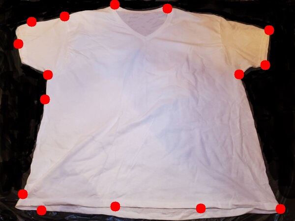
We’ll start with this t-shirt above. Save that image to some folder on your computer.
Now, in the same folder you saved that image above (we’ll call the file tshirt.jpg), open up a new Python program.
Name the program draw_contour.py.
Write the following code:
# Project: How To Draw Contours Around Objects Using OpenCV
# Author: Addison Sears-Collins
# Date created: October 7, 2020
# Reference: https://stackoverflow.com/questions/58405171/how-to-find-the-extreme-corner-point-in-image

import cv2 # OpenCV library
import numpy as np # NumPy scientific computing library

# Read the image
image = cv2.imread("tshirt.jpg")

# Convert the image to grayscale
gray = cv2.cvtColor(image, cv2.COLOR_BGR2GRAY)

# Convert the image to black and white.
# Modify the threshold (e.g. 75 for tshirt.jpg) accordingly depending on how to output looks.
# If you have a dark item on a light background, use cv2.THRESH_BINARY_INV and consider
# changing the lower color threshold to 115.
thresh = cv2.threshold(gray, 75, 255, cv2.THRESH_BINARY)[1]
#thresh = cv2.threshold(gray, 115, 255, cv2.THRESH_BINARY_INV)[1]

# Create a kernel (i.e. a small matrix)
kernel = np.ones((5,5),np.uint8)

# Use the kernel to perform morphological opening
thresh = cv2.morphologyEx(thresh, cv2.MORPH_OPEN, kernel)

# If you have a dark item on a light background, uncomment this line.
#thresh = cv2.morphologyEx(thresh, cv2.MORPH_CLOSE, kernel)

# Find the contours
cnts = cv2.findContours(thresh, cv2.RETR_EXTERNAL, cv2.CHAIN_APPROX_SIMPLE)
cnts = cnts[0] if len(cnts) == 2 else cnts[1]

# Create a blank image
blank_image = np.ones((450,600,3), np.uint8)

# Set the minimum area for a contour
min_area = 5000

# Draw the contours on the original image and the blank image
for c in cnts:
    area = cv2.contourArea(c)
    if area > min_area:
        cv2.drawContours(image,[c], 0, (36,255,12), 2)
        cv2.drawContours(blank_image,[c], 0, (255,255,255), 2)

# Conver the blank image to grayscale for corner detection
gray = cv2.cvtColor(blank_image, cv2.COLOR_BGR2GRAY)

# Detect corners using the contours
corners = cv2.goodFeaturesToTrack(image=gray,maxCorners=25,qualityLevel=0.20,minDistance=50) # Determines strong corners on an image

# Draw the corners on the original image
for corner in corners:
    x,y = corner.ravel()
    cv2.circle(image,(x,y),10,(0,0,255),-1)

 # Display the image
image_copy = cv2.imread("tshirt.jpg")
cv2.imshow('original image', image_copy)
cv2.imshow('image with contours and corners', image)
cv2.imshow('blank_image with contours', blank_image)

# Save the image that has the contours and corners
cv2.imwrite('contour_tshirt.jpg', image)

# Save the image that has just the contours
cv2.imwrite('contour_tshirt_blank_image.jpg', blank_image)

# Exit OpenCV
if cv2.waitKey(0) & 0xff == 27:
    cv2.destroyAllWindows()
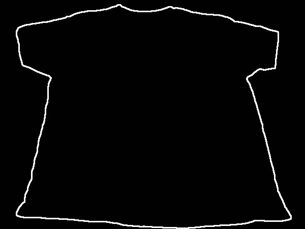
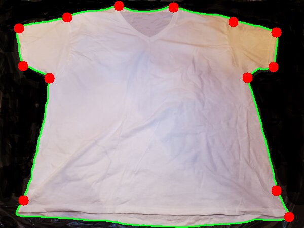
Run the code. Here is what you should see:
Just the contour.
The contour with corner points.
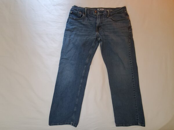
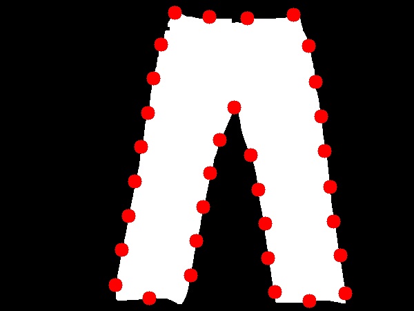
Detecting Corners on Jeans
To detect corners on jeans, you’ll need to make the changes mentioned in the code. This is because the jeans are a dark object on a light background (in contrast to a light object on a dark background in the case of the t-shirt).
Let’s draw a contour around the pair of jeans.
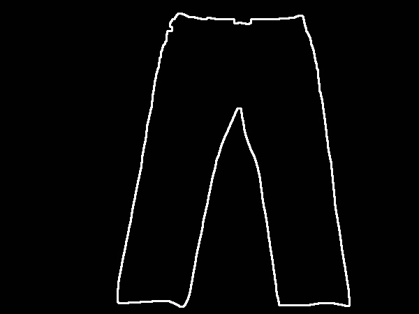
Here is the input image (jeans.jpg):
Change the fileName variable in your code so that it is assigned the name of the image (‘jeans.jpg’).
In this tutorial, we will write a program to detect corners on random objects.
Our goal is to build an early prototype of a vision system that can make it easier and faster for robots to identify potential grasp points on unknown objects.
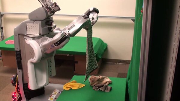
Real-World Applications
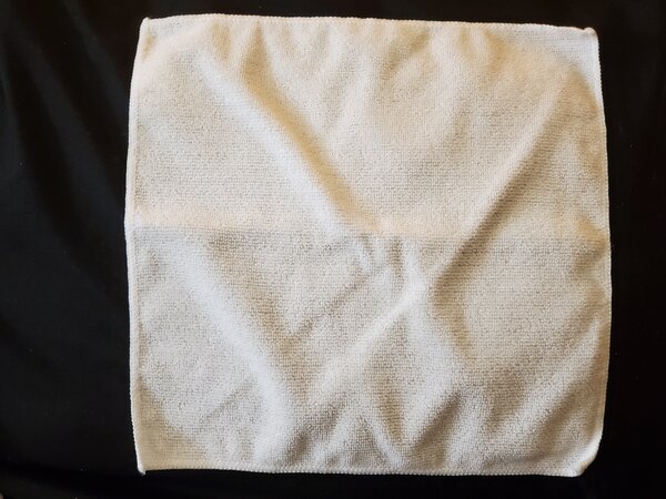
The first real-world application that comes to mind is Dr. Pieter Abbeel (a famous robotics professor at UC Berkley) and his laundry-folding robot.
Dr. Abbeel used the Harris Corner Detector algorithm as a baseline for evaluating how well the robot was able to identify potential grasp points on a variety of laundry items. You can check out his paper at this link.
Source: YouTube (Credit to Berkeley AI Research lab)
If the robot can identify where to grasp a towel, for example, inverse kinematics can then be calculated so the robot can move his arm so that the gripper (i.e. end effector) grasps the corner of the towel to begin the folding process.
Create a program that can detect corners on an unknown object using the Harris Corner Detector algorithm.
Detecting Corners on Jeans
We’ll start with this pair of jeans above. Save that image to some folder on your computer.
Now, in the same folder you saved that image above (we’ll call the file jeans.jpg), open up a new Python program.
Name the program harris_corner_detection.py.
Write the following code:
# Project: Detect the Corners of Objects Using Harris Corner Detector
# Author: Addison Sears-Collins
# Date created: October 7, 2020
# Reference: https://stackoverflow.com/questions/7263621/how-to-find-corners-on-a-image-using-opencv/50556944

import cv2 # OpenCV library
import numpy as np # NumPy scientific computing library
import math # Mathematical functions

# The file name of your image goes here
fileName = 'jeans.jpg'

# Read the image file
img = cv2.imread(fileName)

# Convert the image to grayscale
gray = cv2.cvtColor(img,cv2.COLOR_BGR2GRAY)

######## The code in this block is optional #########
## Turn the image into a black and white image and remove noise
## using opening and closing

#gray = cv2.threshold(gray, 75, 255, cv2.THRESH_BINARY)[1]

#kernel = np.ones((5,5),np.uint8)

#gray = cv2.morphologyEx(gray, cv2.MORPH_OPEN, kernel)
#gray = cv2.morphologyEx(gray, cv2.MORPH_CLOSE, kernel)

## To create a black and white image, it is also possible to use OpenCV's
## background subtraction methods to locate the object in a real-time video stream
## and remove shadows.
## See the following links for examples
## (e.g. Absolute Difference method, BackgroundSubtractorMOG2, etc.):
## https://automaticaddison.com/real-time-object-tracking-using-opencv-and-a-webcam/
## https://automaticaddison.com/motion-detection-using-opencv-on-raspberry-pi-4/

############### End optional block ##################

# Apply a bilateral filter.
# This filter smooths the image, reduces noise, while preserving the edges
bi = cv2.bilateralFilter(gray, 5, 75, 75)

# Apply Harris Corner detection.
# The four parameters are:
#   The input image
#   The size of the neighborhood considered for corner detection
#   Aperture parameter of the Sobel derivative used.
#   Harris detector free parameter
#   --You can tweak this parameter to get better results
#   --0.02 for tshirt, 0.04 for washcloth, 0.02 for jeans, 0.05 for contour_thresh_jeans
#   Source: https://docs.opencv.org/3.4/dc/d0d/tutorial_py_features_harris.html
dst = cv2.cornerHarris(bi, 2, 3, 0.02)

# Dilate the result to mark the corners
dst = cv2.dilate(dst,None)

# Create a mask to identify corners
mask = np.zeros_like(gray)

# All pixels above a certain threshold are converted to white
mask[dst>0.01*dst.max()] = 255

# Convert corners from white to red.
#img[dst > 0.01 * dst.max()] = [0, 0, 255]

# Create an array that lists all the pixels that are corners
coordinates = np.argwhere(mask)

# Convert array of arrays to lists of lists
coordinates_list = [l.tolist() for l in list(coordinates)]

# Convert list to tuples
coordinates_tuples = [tuple(l) for l in coordinates_list]

# Create a distance threshold
thresh = 50

# Compute the distance from each corner to every other corner.
def distance(pt1, pt2):
    (x1, y1), (x2, y2) = pt1, pt2
    dist = math.sqrt( (x2 - x1)**2 + (y2 - y1)**2 )
    return dist

# Keep corners that satisfy the distance threshold
coordinates_tuples_copy = coordinates_tuples
i = 1
for pt1 in coordinates_tuples:
    for pt2 in coordinates_tuples[i::1]:
        if(distance(pt1, pt2) < thresh):
            coordinates_tuples_copy.remove(pt2)
    i+=1

# Place the corners on a copy of the original image
img2 = img.copy()
for pt in coordinates_tuples:
    print(tuple(reversed(pt))) # Print corners to the screen
    cv2.circle(img2, tuple(reversed(pt)), 10, (0, 0, 255), -1)
cv2.imshow('Image with 4 corners', img2)
cv2.imwrite('harris_corners_jeans.jpg', img2)

# Exit OpenCV
if cv2.waitKey(0) & 0xff == 27:
    cv2.destroyAllWindows()
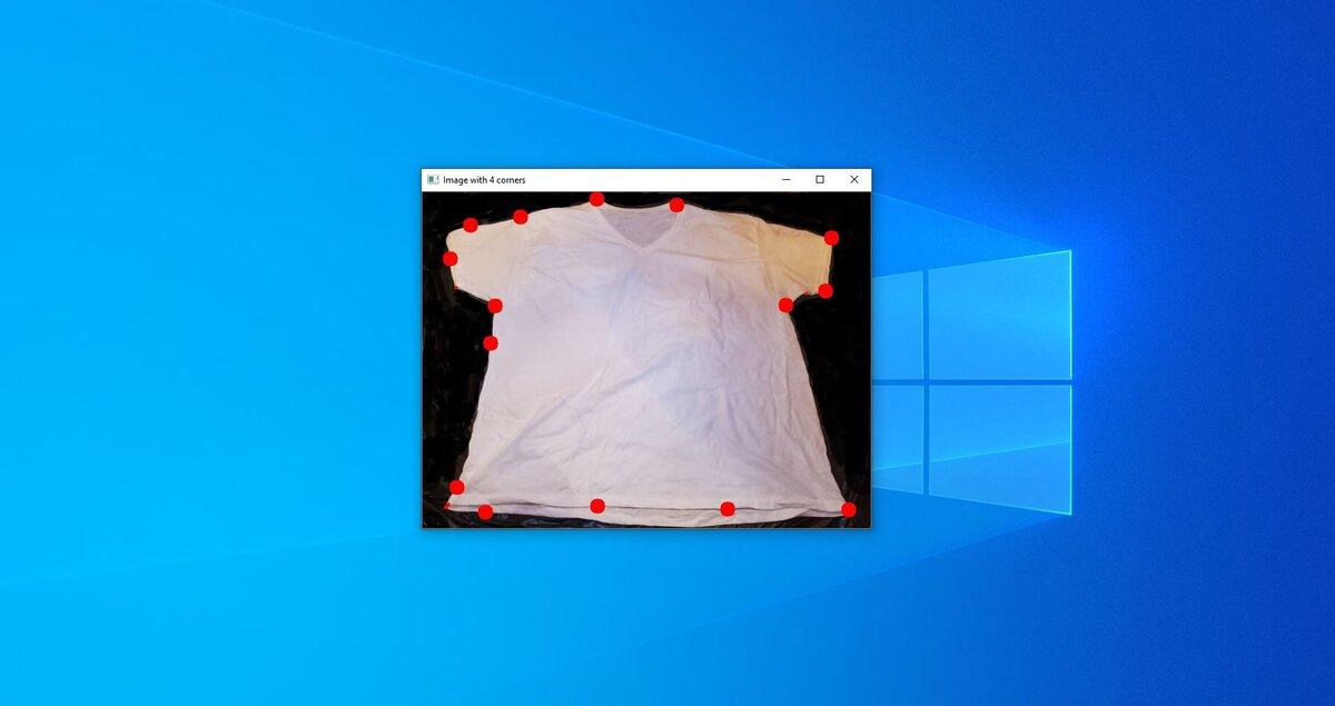
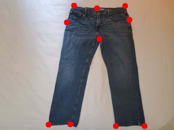
Run the code. Here is what you should see:
Now, if you uncomment the optional block in the code, you will see a window that pops up that shows a binary black and white image of the jeans. The purpose of the optional block of code is to remove some of the noise that is present in the input image.
Notice how when we remove the noise, we get a lot more potential grasp points (i.e. corners).
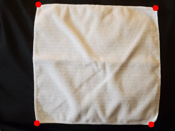
Detecting Corners on a T-Shirt
To detect corners on a t-shirt, you’ll need to tweak the fourth parameter on this line of the code. I use 0.02 typically, but you can try another value like 0.04:
# 0.02 for tshirt, 0.04 for washcloth, 0.02 for jeans, 0.05 for contour_thresh_jeans
#   Source: https://docs.opencv.org/3.4/dc/d0d/tutorial_py_features_harris.html
dst = cv2.cornerHarris(bi, 2, 3, 0.02)
Let’s detect the corners on an ordinary t-shirt.
Here is the input image (tshirt.jpg):
Change the fileName variable in your code so that it is assigned the name of the image (‘tshirt.jpg’).
In this tutorial, we will learn how to create a publisher and a subscriber node in ROS2 (Foxy Fitzroy…the latest version of ROS2) from scratch.
Requirements
We’ll create three separate nodes:
A node that publishes the coordinates of an object detected by a fictitious camera (in reality, we’ll just publish random (x,y) coordinates of an object to a ROS2 topic).
A program that converts the coordinates of the object from the camera reference frame to the (fictitious) robotic arm base frame.
A node that publishes the coordinates of the object with respect to the robotic arm base frame.
I thought this example would be more fun and realistic than the “hello world” example commonly used to teach people how to write ROS subscriber and publisher nodes.
Real-World Applications
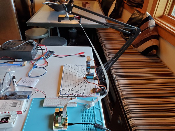
Two degree of freedom robotic arm powered by Arduino with an overhead Raspberry Pi camera. With some additions and modifications, this system could be integrated with ROS2 using the code we’ll develop in this tutorial.
A real-world application of what we’ll accomplish in this tutorial would be a pick and place task where a robotic arm needs to pick up an object from one location and place it in another (e.g. factory, warehouse, etc.).
With some modifications to the code in this tutorial, you can create a complete ROS2-powered robotic system that can:
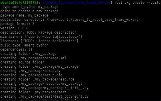
Your package named my_package has now been created.
Build Your Package
Return to the root of your workspace:
cd ~/camera_to_robot_base_frame_ws/
Build all packages in the workspace.
colcon build
Write Node(s)
Open a new terminal window.
Move to the camera_to_robot_base_frame_ws/src/my_package/my_package folder.
cd camera_to_robot_base_frame_ws/src/my_package/my_package
Write this program, and add it to this folder you’re currently in. The name of this file is camera_publisher.py.
This code generates random object coordinates (i.e. x and y location). In a real-world scenario, you would be detecting an object with a camera and then publishing those coordinates to a ROS2 topic.
gedit camera_publisher.py
''' ####################
    Detect an object in a video stream and publish its coordinates
	from the perspective of the camera (i.e. camera reference frame)
	Note: You don't need a camera to run this node. This node just demonstrates how to create
	a publisher node in ROS2 (i.e. how to publish data to a topic in ROS2).
    -------
	Publish the coordinates of the centroid of an object to a topic:
	  /pos_in_cam_frame – The position of the center of an object in centimeter coordinates
    ==================================
    Author: Addison Sears-Collins
    Date: September 28, 2020
    #################### '''

import rclpy # Import the ROS client library for Python
from rclpy.node import Node # Enables the use of rclpy's Node class
from std_msgs.msg import Float64MultiArray # Enable use of the std_msgs/Float64MultiArray message type
import numpy as np # NumPy Python library
import random # Python library to generate random numbers

class CameraPublisher(Node):
  """
  Create a CameraPublisher class, which is a subclass of the Node class.
  The class publishes the position of an object every 3 seconds.
  The position of the object are the x and y coordinates with respect to
  the camera frame.
  """

  def __init__(self):
    """
	Class constructor to set up the node
    """

    # Initiate the Node class's constructor and give it a name
    super().__init__('camera_publisher')

    # Create publisher(s)

    # This node publishes the position of an object every 3 seconds.
    # Maximum queue size of 10.
    self.publisher_position_cam_frame = self.create_publisher(Float64MultiArray, '/pos_in_cam_frame', 10)

    # 3 seconds
    timer_period = 3.0
    self.timer = self.create_timer(timer_period, self.get_coordinates_of_object)
    self.i = 0	# Initialize a counter variable

    # Centimeter to pixel conversion factor
    # Assume we measure 36.0 cm across the width of the field of view of the camera.
    # Assume camera is 640 pixels in width and 480 pixels in height
    self.CM_TO_PIXEL = 36.0 / 640

  def get_coordinates_of_object(self):
    """
    Callback function.
    This function gets called every 3 seconds.
	We locate an object using the camera and then publish its coordinates to ROS2 topics.
    """
    # Center of the bounding box that encloses the detected object.
    # This is in pixel coordinates.
    # Since we don't have an actual camera and an object to detect,
    # we generate random pixel locations.
    # Assume x (width) can go from 0 to 640 pixels, and y (height) can go from 0 to 480 pixels
    x = random.randint(250,450)   # Generate a random integer from 250 to 450 (inclusive)
    y = random.randint(250,450)   # Generate a random integer from 250 to 450 (inclusive)

    # Calculate the center of the object in centimeter coordinates
    # instead of pixel coordinates
    x_cm = x * self.CM_TO_PIXEL
    y_cm = y * self.CM_TO_PIXEL

    # Store the position of the object in a NumPy array
    object_position = [x_cm, y_cm]

    # Publish the coordinates to the topic
    self.publish_coordinates(object_position)

    # Increment counter variable
    self.i += 1

  def publish_coordinates(self,position):
    """
    Publish the coordinates of the object to ROS2 topics
    :param: The position of the object in centimeter coordinates [x , y]
    """
    msg = Float64MultiArray() # Create a message of this type
    msg.data = position # Store the x and y coordinates of the object
    self.publisher_position_cam_frame.publish(msg) # Publish the position to the topic

def main(args=None):

  # Initialize the rclpy library
  rclpy.init(args=args)

  # Create the node
  camera_publisher = CameraPublisher()

  # Spin the node so the callback function is called.
  # Publish any pending messages to the topics.
  rclpy.spin(camera_publisher)

  # Destroy the node explicitly
  # (optional - otherwise it will be done automatically
  # when the garbage collector destroys the node object)
  camera_publisher.destroy_node()

  # Shutdown the ROS client library for Python
  rclpy.shutdown()

if __name__ == '__main__':
  main()
Save the file and close it.
Now change the permissions on the file.
chmod +x camera_publisher.py
Let’s add a program (this isn’t a ROS2 node…it’s just a helper program that performs calculations) that will be responsible for converting the object’s coordinates from the camera reference frame to the to robot base frame. We’ll call it coordinate_transform.py.
gedit coordinate_transform.py
''' ####################
    Convert camera coordinates to robot base frame coordinates
    ==================================
    Author: Addison Sears-Collins
    Date: September 28, 2020
    #################### '''

import numpy as np
import random # Python library to generate random numbers

class CoordinateConversion(object):
  """
  Parent class for coordinate conversions
  All child classes must implement the convert function.
  Every class in Python is descended from the object class
  class CoordinateConversion == class CoordinateConversion(object)
  This class is a superclass, a general class from which
  more specialized classes (e.g. CameraToRobotBaseConversion) can be defined.
  """
  def convert(self, frame_coordinates):
    """
    Convert between coordinate frames

    Input
      :param frame_coordinates: Coordinates of the object in a reference frame (x, y, z, 1)

    Output
      :return: new_frame_coordinates: Coordinates of the object in a new reference frame (x, y, z, 1)

    """
    # Any subclasses that inherit this superclass CoordinateConversion must implement this method.
    raise NotImplementedError


class CameraToRobotBaseConversion(CoordinateConversion):
  """
  Convert camera coordinates to robot base frame coordinates
  This class is a subclass that inherits the methods from the CoordinateConversion class.
  """

  def __init__(self,rot_angle,x_disp,y_disp,z_disp):
    """
    Constructor for the CameraToRobotBaseConversion class. Sets the properties.

    Input
      :param rot_angle: Angle between axes in degrees
      :param x_disp: Displacement between coordinate frames in the x direction in centimeters
      :param y_disp: Displacement between coordinate frames in the y direction in centimeters
      :param z_disp: Displacement between coordinate frames in the z direction in centimeters

    """
    self.angle = np.deg2rad(rot_angle) # Convert degrees to radians
    self.X = x_disp
    self.Y = y_disp
    self.Z = z_disp

  def convert(self, frame_coordinates):
    """
    Convert camera coordinates to robot base frame coordinates

    Input
      :param frame_coordinates: Coordinates of the object in the camera reference frame (x, y, z, 1) in centimeters

    Output
      :return: new_frame_coordinates: Coordinates of the object in the robot base reference frame (x, y, z, 1) in centimeters

    """
    # Define the rotation matrix from the robotic base frame (frame 0)
    # to the camera frame (frame c).
    rot_mat_0_c = np.array([[1, 0, 0],
                            [0, np.cos(self.angle), -np.sin(self.angle)],
                            [0, np.sin(self.angle), np.cos(self.angle)]])

    # Define the displacement vector from frame 0 to frame c
    disp_vec_0_c = np.array([[self.X],
                             [self.Y],
                             [self.Z]])

    # Row vector for bottom of homogeneous transformation matrix
    extra_row_homgen = np.array([[0, 0, 0, 1]])

    # Create the homogeneous transformation matrix from frame 0 to frame c
    homgen_0_c = np.concatenate((rot_mat_0_c, disp_vec_0_c), axis=1) # side by side
    homgen_0_c = np.concatenate((homgen_0_c, extra_row_homgen), axis=0) # one above the other

    # Coordinates of the object in base reference frame
    new_frame_coordinates = homgen_0_c @ frame_coordinates

    return new_frame_coordinates


def main():
  """
  This code is used to test the methods implemented above.
  """

  # Define the displacement from frame base frame of robot to camera frame in centimeters
  x_disp = -17.8
  y_disp = 24.4
  z_disp = 0.0
  rot_angle = 180 # angle between axes in degrees

  # Create a CameraToRobotBaseConversion object
  cam_to_robo = CameraToRobotBaseConversion(rot_angle, x_disp, y_disp, z_disp)

  # Centimeter to pixel conversion factor
  # I measured 36.0 cm across the width of the field of view of the camera.
  CM_TO_PIXEL = 36.0 / 640

  print(f'Detecting an object for 3 seconds')
  dt = 0.1 # Time interval
  t = 0    # Set starting time
  while t<3:
    t = t + dt

    # This is in pixel coordinates.
	# Since we don't have an actual camera and an object to detect,
	# we generate random pixel locations.
	# Assume x (width) can go from 0 to 640 pixels, and y (height) can go from 0 to 480 pixels
    x = random.randint(250,450)   # Generate a random integer from 250 to 450 (inclusive)
    y = random.randint(250,450)   # Generate a random integer from 250 to 450 (inclusive)

    # Calculate the center of the object in centimeter coordinates
    # instead of pixel coordinates
    x_cm = x * CM_TO_PIXEL
    y_cm = y * CM_TO_PIXEL

    # Coordinates of the object in the camera reference frame
    cam_ref_coord = np.array([[x_cm],
                              [y_cm],
                              [0.0],
                              [1]])

    robot_base_frame_coord = cam_to_robo.convert(cam_ref_coord) # Return robot base frame coordinates

    text = "x: " + str(robot_base_frame_coord[0][0]) + ", y: " + str(robot_base_frame_coord[1][0])
    print(f'{t}:{text}') # Display time stamp and coordinates

if __name__ == '__main__':
  main()
Save the file and close it.
Now change the permissions on the file.
chmod +x coordinate_transform.py
Now we’ll add one more node. This node will be responsible for receiving the coordinates of an object in the camera reference frame (these coordinates are published to the ‘/pos_in_cam_frame’ topic by camera_publisher.py), using coordinate_transform.py to convert those coordinates to the robotic arm base frame, and finally publishing these transformed coordinates to the ‘/pos_in_robot_base_frame’ topic.
Name this node robotic_arm_publishing_subscriber.py.
gedit robotic_arm_publishing_subscriber.py
''' ####################
    Receive (i.e. subscribe) coordinates of an object in the camera reference frame, and
	publish those coordinates in the robotic arm base frame.
    -------
	Publish the coordinates of the centroid of an object to topic:
	  /pos_in_robot_base_frame – The x and y position of the center of an object in centimeter coordinates
    ==================================
    Author: Addison Sears-Collins
    Date: September 28, 2020
    #################### '''

import rclpy # Import the ROS client library for Python
from rclpy.node import Node # Enables the use of rclpy's Node class
from std_msgs.msg import Float64MultiArray # Enable use of the std_msgs/Float64MultiArray message type
import numpy as np # NumPy Python library
from .coordinate_transform import CameraToRobotBaseConversion

class PublishingSubscriber(Node):
  """
  Create a PublishingSubscriber class, which is a subclass of the Node class.
  This class subscribes to the x and y coordinates of an object in the camera reference frame.
  The class then publishes the x and y coordinates of the object in the robot base frame.
  """

  def __init__(self):
    """
	Class constructor to set up the node
    """

    # Initiate the Node class's constructor and give it a name
    super().__init__('publishing_subscriber')

    # Create subscriber(s)

    # The node subscribes to messages of type std_msgs/Float64MultiArray, over a topic named:
    #   /pos_in_cam_frame
    # The callback function is called as soon as a message is received.
    # The maximum number of queued messages is 10.
    self.subscription_1 = self.create_subscription(
      Float64MultiArray,
      '/pos_in_cam_frame',
      self.pos_received,
      10)
    self.subscription_1  # prevent unused variable warning

    # Create publisher(s)

    # This node publishes the position in robot frame coordinates.
    # Maximum queue size of 10.
    self.publisher_pos_robot_frame = self.create_publisher(Float64MultiArray, '/pos_in_robot_base_frame', 10)

    # Define the displacement from frame base frame of robot to camera frame in centimeters
    x_disp = -17.8
    y_disp = 24.4
    z_disp = 0.0
    rot_angle = 180 # angle between axes in degrees

    # Create a CameraToRobotBaseConversion object
    self.cam_to_robo = CameraToRobotBaseConversion(rot_angle, x_disp, y_disp, z_disp)

  def pos_received(self, msg):
    """
    Callback function.
    This function gets called as soon as the position of the object is received.
    :param: msg is of type std_msgs/Float64MultiArray
    """
    object_position = msg.data

    # Coordinates of the object in the camera reference frame in centimeters
    cam_ref_coord = np.array([[object_position[0]],
                              [object_position[1]],
                              [0.0],
                              [1]])

    robot_base_frame_coord = self.cam_to_robo.convert(cam_ref_coord) # Return robot base frame coordinates

    # Capture the object's desired position (x, y)
    object_position = [robot_base_frame_coord[0][0], robot_base_frame_coord[1][0]]

    # Publish the coordinates to the topics
    self.publish_position(object_position)

  def publish_position(self,object_position):
    """
    Publish the coordinates of the object with respect to the robot base frame.
    :param: object position [x, y]
    """
    msg = Float64MultiArray() # Create a message of this type
    msg.data = object_position # Store the object's position
    self.publisher_pos_robot_frame.publish(msg) # Publish the position to the topic

def main(args=None):

  # Initialize the rclpy library
  rclpy.init(args=args)

  # Create the node
  publishing_subscriber = PublishingSubscriber()

  # Spin the node so the callback function is called.
  # Pull messages from any topics this node is subscribed to.
  # Publish any pending messages to the topics.
  rclpy.spin(publishing_subscriber)

  # Destroy the node explicitly
  # (optional - otherwise it will be done automatically
  # when the garbage collector destroys the node object)
  publishing_subscriber.destroy_node()

  # Shutdown the ROS client library for Python
  rclpy.shutdown()

if __name__ == '__main__':
  main()
Save the file and close it.
Now change the permissions on the file.
chmod +x robotic_arm_publishing_subscriber.py
Add Dependencies
Navigate one level back.
cd ..
You are now in the camera_to_robot_base_frame_ws/src/my_package/ directory.
Type
ls
You should see the setup.py, setup.cfg, and package.xml files.
Open package.xml with your text editor.
gedit package.xml
Fill in the <description>, <maintainer>, and <license> tags.
  <name>my_package</name>
  <version>0.0.0</version>
  <description>Converts camera coordinates to robotic arm base frame coordinates</description>
  <maintainer email="example@automaticaddison.com">Addison Sears-Collins</maintainer>
  <license>All Rights Reserved.</license>
Add a new line after the ament_python build_type dependency, and add the following dependencies which will correspond to other packages the packages in this workspace needs (this will be in your node’s import statements):
<exec_depend>rclpy</exec_depend>
<exec_depend>std_msgs</exec_depend>
This let’s the system know that this package needs the rclpy and std_msgs packages when its code is executed.
Save the file and close it.
Add an Entry Point
Now we need to add the entry points for the node(s) by opening the setup.py file.
gedit setup.py
Make sure to modify the entry_points block of code so that it looks like this:
Now, build your package by first moving to the src folder.
cd src
Then build the package.
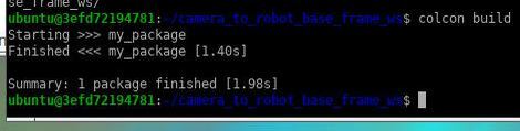
colcon build
You should get a message that says:
“Summary: 1 package finished [<time it took in seconds>]”
If you get errors, go to your Python programs and check for errors. Python is sensitive to indentation (tabs and spaces), so make sure the spacing of the code is correct (go one line at a time through the code).
The programs are located in this folder.
cd camera_to_robot_base_frame_ws/src/my_package/my_package
After you make changes, build the package again.
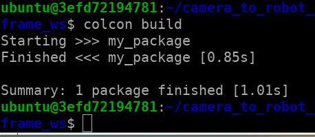
cd ~/camera_to_robot_base_frame_ws
colcon build
You should see this message when everything build successfully:
Open a new terminal tab.
Run the nodes:
ros2 run my_packagecamera_publisher
In another terminal tab:
ros2 run robotic_arm_publishing_subscriber
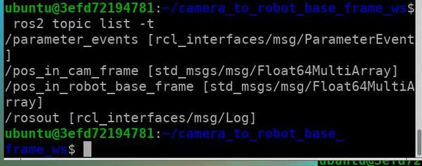
Open a new terminal tab, and move to the root directory of the workspace.
cd ~/camera_to_robot_base_frame_ws
List the active topics.
ros2 topic list -t
To listen to any topic, type:
ros2 topic echo /topic_name
Where you replace “/topic_name” with the name of the topic.
For example:
ros2 topic echo /pos_in_cam_frame
You should see the (x, y) coordinates of the object (in the camera reference frame) printed to the screen.
In another terminal, you can type:
ros2 topic echo /pos_in_robot_base_frame
You should see the (x, y) coordinates of the object (in the robot base frame) printed to the screen.
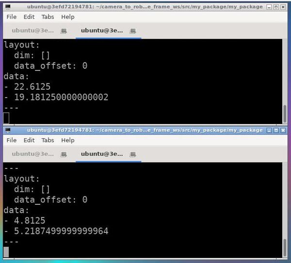
Here is how my terminal windows look. The camera coordinates in centimeters are on top, and the robot base frame coordinates are on the bottom.
When you’ve had enough, type Ctrl+C in each terminal tab to stop the nodes from spinning.
Zip the Workspace for Distribution
If you ever want to zip the whole workspace and send it to someone, open a new terminal window.
Move to the directory containing your workspace.
cd ~/camera_to_robot_base_frame_ws
cd ..
zip -r camera_to_robot_base_frame_ws.zip camera_to_robot_base_frame_ws